Exam 12: Multiple Regression and Model Building

The first-order model below was fit to a set of data. $E ( y ) = \beta _ { 0 } + \beta _ { 1 } x _ { 1 } + \beta _ { 2 } x _ { 2 }$ Explain how to determine if the constant variance assumption is satisfied.

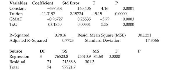
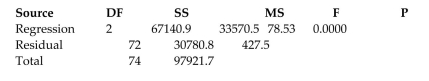
A study of the top MBA programs attempted to predict the average starting salary (in $1000ʹs)of graduates of the program based on the amount of tuition (in $1000ʹs)charged by the program and The average GMAT score of the programʹs students. The results of a regression analysis based on a Sample of 75 MBA programs is shown below: Least Squares Linear Regression of Salary Predictor Cases Included $75 \quad$ Missing Cases 0 The global- $\mathrm { f }$ test statistic is shown on the printout to be the value $\mathrm { F } = 84.68$ . Interpret this value.

A study of the top MBA programs attempted to predict the average starting salary (in $1000ʹs)of graduates of the program based on the amount of tuition (in $1000ʹs)charged by the program and The average GMAT score of the programʹs students. The results of a regression analysis based on a Sample of 75 MBA programs is shown below: Least Squares Linear Regression of Salary Predictor The model was then used to create $95 \%$ confidence and prediction intervals for $y$ and for $E ( Y )$ when the tuition charged by the MBA program was $\$ 75,000$ and the GMAT score was 675 . The results are shown here: $95 \%$ confidence interval for $\mathrm { E } ( \mathrm { Y } )$ : $( \$ 126,610 , \$ 136,640 )$ $95 \%$ prediction interval for $Y$ : $( \$ 90,113 , \$ 173,160 )$ Which of the following interpretations is correct if you want to use the model to estimate $Y$ for a single MBA program?

A statistics professor gave three quizzes leading up to the first test in his class. The quiz grades and test grade for each of eight students are given in the table. 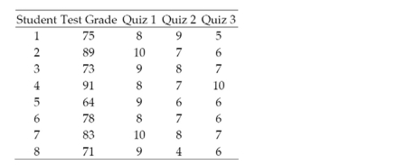The professor fit a first-order model to the data that he intends to use to predict a student 's grade on the first test using that student's grades on the first three quizzes. Test the null hypothesis $H _ { 0 } : \beta _ { 1 } = \beta _ { 2 } = \beta _ { 3 } = 0$ against the alternative hypothesis $H _ { \mathrm { a } } :$ at least one $\beta _ { i } \neq 0$ . Use $\alpha = , 05$ . Interpret the result.

A study of the top MBA programs attempted to predict the average starting salary (in $1000ʹs)of graduates of the program based on the amount of tuition (in $1000ʹs)charged by the program and The average GMAT score of the programʹs students. The results of a regression analysis based on a Sample of 75 MBA programs is shown below: Least Squares Linear Regression of Salary $\text { Predictor }$ The model was then used to create $95 \%$ confidence and prediction intervals for $y$ and for $E ( Y )$ when the tuition charged by the MBA program was $\$ 75,000$ and the GMAT score was 675 . The results are shown here: $95 \%$ confidence interval for $\mathrm { E } ( \mathrm { Y } ) : ( \$ 126,610 , \$ 136,640 )$ $95 \%$ prediction interval for $\mathrm { Y } : ( \$ 90,113 , \$ 173,160 )$ Which of the following interpretations is correct if you want to use the model to estimate $E ( Y )$ for all MBA programs?

In any production process in which one or more workers are engaged in a variety of tasks, the total time spent in production varies as a function of the size of the workpool and the level of output of the various activities. In a large metropolitan department store, it is believed that the number of man-hours worked $( y )$ per day by the clerical staff depends on the number of pieces of mail processed per day $\left( x _ { 1 } \right)$ and the number of checks cashed per day $\left( x _ { 2 } \right)$ . Data collected for $n = 20$ working days were used to fit the model: $E ( y ) = \beta _ { 0 } + \beta _ { 1 } x _ { 1 } + \beta _ { 2 } x _ { 2 }$ A printout for the analysis follows: Analysis of Variance SOURCE DF SS MS F VALUE PROB > F 2 7089.06512 3544.53256 13.267 0.0003 MODEL 17 4541.72142 267.16008 ERROR 19 11630.78654 ROOT MSE 16.34503 R-SQUARE 0.6095 DEP MEAN 93.92682 ADJ R-SQ 0.5636 C.V. 17.40188 PARAMETER STANDARD T FOR 0: VARIABLE DF ESTIMATE ERROR PARAMETER =0 PROB >|| INTERCEPT 1 114.420972 18.68485744 X1 1 -0.007102 0.00171375 6.124 0.0001 X2 1 0.037290 0.02043937 -4.144 0.0007 1.824 0.0857 OBS X1 X2 Actual Value Predict Value Residual Lower 95\% CL Predict Upper 95\% CL Predict 7781 644 74.707 83.175 -8.468 47.224 119.126 Test to determine if there is a positive linear relationship between the number of man-hours worked, $y$ , and the number of checks cashed per day, $x _ { 2 }$ . Use $\alpha = .05$ .

The value of $R ^ { 2 }$ is only useful when the number of data points is substantially larger than the number of $\beta$ parameters in the model.

An elections officer wants to model voter turnout (y)in a precinct as a function of the type of precinct. Consider the model relating mean voter turnout, $E ( y )$ , to precinct type: 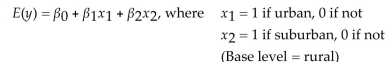The $p$ -value for the test $H _ { 0 } : \beta _ { 1 } = \beta _ { 2 } = 0$ is .14. Interpret the result.

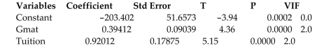
Retail price data for n = 60 hard disk drives were recently reported in a computer magazine. 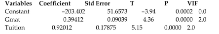Three variables were recorded for each hard disk drive: $\mathrm { y } =$ Retail PRICE (measured in dollars) $\mathrm { x } _ { 1 }$ = Microprocessor SPEED (measured in megahertz) (Values in sample range from 10 to 40 ) $\mathrm { x } _ { 2 } = \mathrm { CHIP }$ size (measured in computer processing units) (Values in sample range from 286 to 486 ) A first-order regression model was fit to the data. Part of the printout follows: 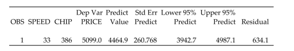Interpret the $95 \%$ prediction interval for $y$ when $x _ { 1 } = 33$ and $x _ { 2 } = 386$ .

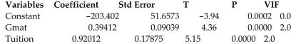
A study of the top MBA programs attempted to predict the average starting salary (in $1000ʹs)of graduates of the program based on the amount of tuition (in $1000ʹs)charged by the program and The average GMAT score of the programʹs students. The results of a regression analysis based on a Sample of 75 MBA programs is shown below: Least Squares Linear Regression of Salary Predictor Interpret the $p$ -value for the global $f$ -test shown on the printout.

A graphing calculator was used to fit the model $E ( y ) = \beta _ { 0 } + \beta _ { 1 } x + \beta _ { 2 } x ^ { 2 }$ to a set of data. The resulting screen is shown below. 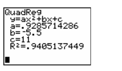Which number on the screen represents the estimator of $\beta _ { 2 }$ ?