Deck 16: Time-Series Forecasting and Index Numbers
Full screen (f)
Question
Question
Question
Question
Question
Question
Question
Question
Question
Question
Question
Question
Question
Question
Question
Question
Question
Question
Question
Question
Question
Question
Question
After estimating a trend model for annual time-series data, you obtain the following residual plot against time, the problem with your model is that 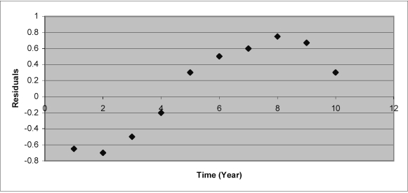
A) the trend component has not been accounted for.
B) the irregular component has not been accounted for.
C) the cyclical component has not been accounted for.
D) the seasonal component has not been accounted for.
A) the trend component has not been accounted for.
B) the irregular component has not been accounted for.
C) the cyclical component has not been accounted for.
D) the seasonal component has not been accounted for.
Question
Question
Question
Question
Question
Question
Question
Question
Question
Question
Based on the following scatter plot, which of the time- series components is not present in this quarterly time series? 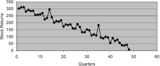
A) trend
B) irregular
C) seasonal
D) cyclical
A) trend
B) irregular
C) seasonal
D) cyclical
Question
Question
Question
Question
Question
Question
Question
Question
Question
Question
Question
Question
Question
TABLE 16-14
Given below are the average prices for three types of energy products in the United States from 1992 to 1995.

Referring to Table 16-14, what are the simple price indexes for electricity, natural gas and fuel oil, respectively, in 1995 using 1992 as the base year?
Given below are the average prices for three types of energy products in the United States from 1992 to 1995.
Referring to Table 16-14, what are the simple price indexes for electricity, natural gas and fuel oil, respectively, in 1995 using 1992 as the base year?
Question
Question
Question
Question
Question
Question
Question
Question
Question
Question
Question
Question
Question
Question
Question
Question
Question
Question
Question
Question
Question
Question
Question
Question
Question
TABLE 16-14
Given below are the average prices for three types of energy products in the United States from 1992 to 1995.
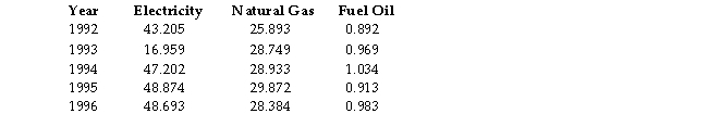
Referring to Table 16-14, what is the Paasche price index for the group of three energy items in 1996 for a family that consumed 13 units of electricity, 26 units of natural gas and 235 units of fuel oil in 1996 using 1992 as the base year?
Given below are the average prices for three types of energy products in the United States from 1992 to 1995.
Referring to Table 16-14, what is the Paasche price index for the group of three energy items in 1996 for a family that consumed 13 units of electricity, 26 units of natural gas and 235 units of fuel oil in 1996 using 1992 as the base year?
Question
TABLE 16-14
Given below are the average prices for three types of energy products in the United States from 1992 to 1995.

Referring to Table 16-14, what are the simple price indexes for electricity, natural gas and fuel oil, respectively, in 1994 using 1996 as the base year?
Given below are the average prices for three types of energy products in the United States from 1992 to 1995.
Referring to Table 16-14, what are the simple price indexes for electricity, natural gas and fuel oil, respectively, in 1994 using 1996 as the base year?
Question
Question
Question
Question
Question
TABLE 16-15
Given below are the prices of a basket of four food items from 1996 to 2000.
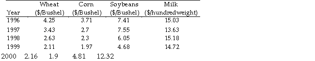
Referring to Table 16-15, what is the Paasche price index for the basket of four food items in 1999 that consisted of 60 bushels of wheat, 40 bushels of corn, 35 bushels of soybeans and 70 hundredweight of milk in 1999 using 1996 as the base year?
Given below are the prices of a basket of four food items from 1996 to 2000.
Referring to Table 16-15, what is the Paasche price index for the basket of four food items in 1999 that consisted of 60 bushels of wheat, 40 bushels of corn, 35 bushels of soybeans and 70 hundredweight of milk in 1999 using 1996 as the base year?
Question
Question
Question

Unlock Deck
Sign up to unlock the cards in this deck!
Unlock Deck
Unlock Deck
1/193
Play
Full screen (f)
Deck 16: Time-Series Forecasting and Index Numbers
1
Which of the following terms describes the up and down movements of a time series that vary both in length and intensity?
A) seasonal component
B) irregular component
C) cyclical component
D) trend
A) seasonal component
B) irregular component
C) cyclical component
D) trend
C
2
The following is the list of MAD statistics for each of the models you have estimated from time-series data: Based on the MAD criterion, the most appropriate model is
A) exponential trend.
B) linear trend.
C) AR(2).
D) quadratic trend.
A) exponential trend.
B) linear trend.
C) AR(2).
D) quadratic trend.
AR(2).
3
TABLE 16-3
The following table contains the number of complaints received in a department store for the first 6 months of last year.
-Referring to Table 16-3, if this series is smoothed using exponential smoothing with a smoothing constant of 1/3, how many terms would it have?
A) 4
B) 6
C) 5
D) 3
The following table contains the number of complaints received in a department store for the first 6 months of last year.
-Referring to Table 16-3, if this series is smoothed using exponential smoothing with a smoothing constant of 1/3, how many terms would it have?
A) 4
B) 6
C) 5
D) 3
6
4
TABLE 16-13
A local store developed a multiplicative time-series model to forecast its revenues in future quarters, using quarterly data on its revenues during the 4-year period from 1998 to 2002. The following is the resulting regression equation:
log10Y^ = 6.102 + 0.012 X - 0.129 Q1 - 0.054 Q2 + 0.098 Q3
where
Y^ is the estimated number of contracts in a quarter
X is the coded quarterly value with X = 0 in the first quarter of 1998.
Q1 is a dummy variable equal to 1 in the first quarter of a year and 0 otherwise.
Q2 is a dummy variable equal to 1 in the second quarter of a year and 0 otherwise.
Q3 is a dummy variable equal to 1 in the third quarter of a year and 0 otherwise.
-Referring to Table 16-13, the estimated quarterly compound growth rate in revenues is around
A) 12%.
B) 28%.
C) 2.8%.
D) 1.2%.
Unlock Deck
Unlock for access to all 193 flashcards in this deck.
Unlock Deck
k this deck
5
Which of the following is not an advantage of exponential smoothing?
A) It enables us to perform more than one-period ahead forecasting.
B) It enables us to smooth out seasonal components.
C) It enables us to perform one-period ahead forecasting.
D) It enables us to smooth out cyclical components.
A) It enables us to perform more than one-period ahead forecasting.
B) It enables us to smooth out seasonal components.
C) It enables us to perform one-period ahead forecasting.
D) It enables us to smooth out cyclical components.
Unlock Deck
Unlock for access to all 193 flashcards in this deck.
Unlock Deck
k this deck
6
Which of the following terms describes the overall long-term tendency of a time series?
A) trend
B) irregular component
C) seasonal component
D) cyclical component
A) trend
B) irregular component
C) seasonal component
D) cyclical component
Unlock Deck
Unlock for access to all 193 flashcards in this deck.
Unlock Deck
k this deck
7
TABLE 16-13
A local store developed a multiplicative time-series model to forecast its revenues in future quarters, using quarterly data on its revenues during the 4-year period from 1998 to 2002. The following is the resulting regression equation:
log10Y^ = 6.102 + 0.012 X - 0.129 Q1 - 0.054 Q2 + 0.098 Q3
where
Y^ is the estimated number of contracts in a quarter
X is the coded quarterly value with X = 0 in the first quarter of 1998.
Q1 is a dummy variable equal to 1 in the first quarter of a year and 0 otherwise.
Q2 is a dummy variable equal to 1 in the second quarter of a year and 0 otherwise.
Q3 is a dummy variable equal to 1 in the third quarter of a year and 0 otherwise.
-Referring to Table 16-13, the best interpretation of the constant 6.102 in the regression equation is
A) the fitted value for the first quarter of 1998, after to seasonal adjustment, is 106.102.
B) the fitted value for the first quarter of 1998, prior to seasonal adjustment, is log10(6.102).
C) the fitted value for the first quarter of 1998, prior to seasonal adjustment, is 106.102.
D) the fitted value for the first quarter of 1998, after to seasonal adjustment, is log10(6.102).
Unlock Deck
Unlock for access to all 193 flashcards in this deck.
Unlock Deck
k this deck
8
TABLE 16-5
A contractor developed a multiplicative time-series model to forecast the number of contracts in future quarters, using quarterly data on number of contracts during the 3-year period from 1996 to 1998. The following is the resulting regression equation:
ln Y^ = 3.37 + 0.117 X - 0.083 Q1 + 1.28 Q2 + 0.617 Q3
where
Y^ is the estimated number of contracts in a quarter
X is the coded quarterly value with X = 0 in the first quarter of 1996.
Q1 is a dummy variable equal to 1 in the first quarter of a year and 0 otherwise.
Q2 is a dummy variable equal to 1 in the second quarter of a year and 0 otherwise.
Q3 is a dummy variable equal to 1 in the third quarter of a year and 0 otherwise.
-Referring to Table 16-5, in testing the coefficient for Q1 in the regression equation (- 0.083), the results were a t-statistic of - 0.66 and an associated p-value of 0.530. Which of the following is the best interpretation of this result?
A) The number of contracts in the first quarter of the year is not significantly different than the number of contracts in an average quarter (? = 0.05).
B) The number of contracts in the first quarter of the year is not significantly different than the number of contracts in the fourth quarter for a given coded quarterly value of X (? = 0.05).
C) The number of contracts in the first quarter of the year is significantly different than the number of contracts in an average quarter (? = 0.05).
D) The number of contracts in the first quarter of the year is significantly different than the number of contracts in the fourth quarter for a given coded quarterly value of X (? = 0.05).
Unlock Deck
Unlock for access to all 193 flashcards in this deck.
Unlock Deck
k this deck
9
TABLE 16-5
A contractor developed a multiplicative time-series model to forecast the number of contracts in future quarters, using quarterly data on number of contracts during the 3-year period from 1996 to 1998. The following is the resulting regression equation:
ln Y^ = 3.37 + 0.117 X - 0.083 Q1 + 1.28 Q2 + 0.617 Q3
where
Y^ is the estimated number of contracts in a quarter
X is the coded quarterly value with X = 0 in the first quarter of 1996.
Q1 is a dummy variable equal to 1 in the first quarter of a year and 0 otherwise.
Q2 is a dummy variable equal to 1 in the second quarter of a year and 0 otherwise.
Q3 is a dummy variable equal to 1 in the third quarter of a year and 0 otherwise.
-Referring to Table 16-5, the best interpretation of the coefficient of X (0.117) in the regression equation is
A) the annually compound growth rate in contracts is around 11.7%.
B) the quarterly compound growth rate in contracts is around 11.7%.
C) the annually compound growth rate in contracts is around 30.92%.
D) the quarterly compound growth rate in contracts is around 30.92%.
Unlock Deck
Unlock for access to all 193 flashcards in this deck.
Unlock Deck
k this deck
10
TABLE 16-5
A contractor developed a multiplicative time-series model to forecast the number of contracts in future quarters, using quarterly data on number of contracts during the 3-year period from 1996 to 1998. The following is the resulting regression equation:
ln Y^ = 3.37 + 0.117 X - 0.083 Q1 + 1.28 Q2 + 0.617 Q3
where Y^ is the estimated number of contracts in a quarter
X is the coded quarterly value with X = 0 in the first quarter of 1996.
Q1 is a dummy variable equal to 1 in the first quarter of a year and 0 otherwise. Q2 is a dummy variable equal to 1 in the second quarter of a year and 0 otherwise. Q3 is a dummy variable equal to 1 in the third quarter of a year and 0 otherwise.
Referring to Table 16-5, to obtain a forecast for the fourth quarter of 1999 using the model, which of the following sets of values should be used in the regression equation?
A) X = 15, Q1 = 1, Q2 = 0, Q3 = 0
B) X = 16, Q1 = 0, Q2 = 0, Q3 = 0
C) X = 16, Q1 = 1, Q2 = 0, Q3 = 0
D) X = 15, Q1 = 0, Q2 = 0, Q3 = 0
Unlock Deck
Unlock for access to all 193 flashcards in this deck.
Unlock Deck
k this deck
11
When using the exponentially weighted moving average for purposes of forecasting rather than smoothing,
A) the next smoothed value becomes the forecast.
B) the current smoothed value becomes the forecast.
C) the previous smoothed value becomes the forecast.
D) none of the above
A) the next smoothed value becomes the forecast.
B) the current smoothed value becomes the forecast.
C) the previous smoothed value becomes the forecast.
D) none of the above
Unlock Deck
Unlock for access to all 193 flashcards in this deck.
Unlock Deck
k this deck
12
TABLE 16-13
A local store developed a multiplicative time-series model to forecast its revenues in future quarters, using quarterly data on its revenues during the 4-year period from 1998 to 2002. The following is the resulting regression equation:
log10Y^ = 6.102 + 0.012 X - 0.129 Q1 - 0.054 Q2 + 0.098 Q3
where
Y^ is the estimated number of contracts in a quarter
X is the coded quarterly value with X = 0 in the first quarter of 1998.
Q1 is a dummy variable equal to 1 in the first quarter of a year and 0 otherwise.
Q2 is a dummy variable equal to 1 in the second quarter of a year and 0 otherwise.
Q3 is a dummy variable equal to 1 in the third quarter of a year and 0 otherwise.
-Referring to Table 16-13, to obtain a forecast for the third quarter of 2003 using the model, which of the following sets of values should be used in the regression equation?
A) X = 22, Q1 = 0, Q2 = 0, Q3 = 0
B) X = 23, Q1 = 0, Q2 = 0, Q3 = 1
C) X = 22, Q1 = 0, Q2 = 0, Q3 = 1
D) X = 23, Q1 = 0, Q2 = 0, Q3 = 0
Unlock Deck
Unlock for access to all 193 flashcards in this deck.
Unlock Deck
k this deck
13
TABLE 16-13
A local store developed a multiplicative time-series model to forecast its revenues in future quarters, using quarterly data on its revenues during the 4-year period from 1998 to 2002. The following is the resulting regression equation:
log10Y^ = 6.102 + 0.012 X - 0.129 Q1 - 0.054 Q2 + 0.098 Q3
where
Y^ is the estimated number of contracts in a quarter
X is the coded quarterly value with X = 0 in the first quarter of 1998.
Q1 is a dummy variable equal to 1 in the first quarter of a year and 0 otherwise.
Q2 is a dummy variable equal to 1 in the second quarter of a year and 0 otherwise.
Q3 is a dummy variable equal to 1 in the third quarter of a year and 0 otherwise.
-Referring to Table 16-13, to obtain a forecast for the first quarter of 2002 using the model, which of the following sets of values should be used in the regression equation?
A) X = 17, Q1 = 1, Q2 = 0, Q3 = 0
B) X = 16, Q1 = 1, Q2 = 0, Q3 = 0
C) X = 16, Q1 = 0, Q2 = 1, Q3 = 0
D) X = 17, Q1 = 0, Q2 = 1, Q3 = 0
Unlock Deck
Unlock for access to all 193 flashcards in this deck.
Unlock Deck
k this deck
14
A model that can be used to make predictions about long-term future values of a time series is
A) exponential trend.
B) linear trend.
C) quadratic trend.
D) all of the above
A) exponential trend.
B) linear trend.
C) quadratic trend.
D) all of the above
Unlock Deck
Unlock for access to all 193 flashcards in this deck.
Unlock Deck
k this deck
15
The overall upward or downward pattern of the data in an annual time series will be contained in the _____component.
A) cyclical
B) irregular
C) seasonal
D) trend
A) cyclical
B) irregular
C) seasonal
D) trend
Unlock Deck
Unlock for access to all 193 flashcards in this deck.
Unlock Deck
k this deck
16
TABLE 16-3
The following table contains the number of complaints received in a department store for the first 6 months of last year.
-Referring to Table 16-3, if a three-term moving average is used to smooth this series, what would be the last calculated term?
A) 126
B) 93
C) 72
D) 114
The following table contains the number of complaints received in a department store for the first 6 months of last year.
-Referring to Table 16-3, if a three-term moving average is used to smooth this series, what would be the last calculated term?
A) 126
B) 93
C) 72
D) 114
Unlock Deck
Unlock for access to all 193 flashcards in this deck.
Unlock Deck
k this deck
17
The effect of an unpredictable, rare event will be contained in the component.
A) trend
B) irregular
C) cyclical
D) seasonal
A) trend
B) irregular
C) cyclical
D) seasonal
Unlock Deck
Unlock for access to all 193 flashcards in this deck.
Unlock Deck
k this deck
18
TABLE 16-13
A local store developed a multiplicative time-series model to forecast its revenues in future quarters, using quarterly data on its revenues during the 4-year period from 1998 to 2002. The following is the resulting regression equation:
log10Y^ = 6.102 + 0.012 X - 0.129 Q1 - 0.054 Q2 + 0.098 Q3
where
Y^ is the estimated number of contracts in a quarter
X is the coded quarterly value with X = 0 in the first quarter of 1998.
Q1 is a dummy variable equal to 1 in the first quarter of a year and 0 otherwise.
Q2 is a dummy variable equal to 1 in the second quarter of a year and 0 otherwise.
Q3 is a dummy variable equal to 1 in the third quarter of a year and 0 otherwise.
-Referring to Table 16-13, the best interpretation of the coefficient of Q2 (- 0.054) in the regression equation is
A) the revenues in the second quarter of a year is approximately 5.4% lower than it would be during the fourth quarter.
B) the revenues in the second quarter of a year is approximately 5.4% lower than the average over all 4 quarters.
C) the revenues in the second quarter of a year is approximately 11.69% lower than the average over all 4 quarters.
D) the revenues in the second quarter of a year is approximately 11.69% lower than it would be during the fourth quarter.
Unlock Deck
Unlock for access to all 193 flashcards in this deck.
Unlock Deck
k this deck
19
TABLE 16-5
A contractor developed a multiplicative time-series model to forecast the number of contracts in future quarters, using quarterly data on number of contracts during the 3-year period from 1996 to 1998. The following is the resulting regression equation:
ln Y^ = 3.37 + 0.117 X - 0.083 Q1 + 1.28 Q2 + 0.617 Q3
where
Y^ is the estimated number of contracts in a quarter
X is the coded quarterly value with X = 0 in the first quarter of 1996.
Q1 is a dummy variable equal to 1 in the first quarter of a year and 0 otherwise.
Q2 is a dummy variable equal to 1 in the second quarter of a year and 0 otherwise.
Q3 is a dummy variable equal to 1 in the third quarter of a year and 0 otherwise.
-Referring to Table 16-5, using the regression equation, which of the following values is the best forecast for the number of contracts in the second quarter of 2000?
A) 391742
B) 144212
C) 4355119
D) 1238797
Unlock Deck
Unlock for access to all 193 flashcards in this deck.
Unlock Deck
k this deck
20
TABLE 16-13
A local store developed a multiplicative time-series model to forecast its revenues in future quarters, using quarterly data on its revenues during the 4-year period from 1998 to 2002. The following is the resulting regression equation:
log10Y^ = 6.102 + 0.012 X - 0.129 Q1 - 0.054 Q2 + 0.098 Q3
where
Y^ is the estimated number of contracts in a quarter
X is the coded quarterly value with X = 0 in the first quarter of 1998.
Q1 is a dummy variable equal to 1 in the first quarter of a year and 0 otherwise.
Q2 is a dummy variable equal to 1 in the second quarter of a year and 0 otherwise.
Q3 is a dummy variable equal to 1 in the third quarter of a year and 0 otherwise.
-Referring to Table 16-13, in testing the significance of the coefficient for Q1 in the regression equation (- 0.129) which has a p-value of 0.492. Which of the following is the best interpretation of this result?
A) The revenues in the first quarter of the year are not significantly different than the revenues in the fourth quarter (? = 0.05).
B) The revenues in the first quarter of the year are significantly different than the revenues in the fourth quarter (? = 0.05).
C) The revenues in the first quarter of the year are significantly different than the revenues in an average quarter (? = 0.05).
D) The revenues in the first quarter of the year are not significantly different than the revenues in an average quarter (? = 0.05).
Unlock Deck
Unlock for access to all 193 flashcards in this deck.
Unlock Deck
k this deck
21
TABLE 16-13
A local store developed a multiplicative time-series model to forecast its revenues in future quarters, using quarterly data on its revenues during the 4-year period from 1998 to 2002. The following is the resulting regression equation:
log10Y^ = 6.102 + 0.012 X - 0.129 Q1 - 0.054 Q2 + 0.098 Q3
where
Y^ is the estimated number of contracts in a quarter
X is the coded quarterly value with X = 0 in the first quarter of 1998.
Q1 is a dummy variable equal to 1 in the first quarter of a year and 0 otherwise.
Q2 is a dummy variable equal to 1 in the second quarter of a year and 0 otherwise.
Q3 is a dummy variable equal to 1 in the third quarter of a year and 0 otherwise.
-Referring to Table 16-13, in testing the significance of the coefficient of X in the regression equation (0.012) which has a p-value of 0.0000. Which of the following is the best interpretation of this result?
A) The quarterly growth rate in revenues is significantly different from 1.2% (? = 0.05).
B) The quarterly growth rate in revenues is significantly different from 0% (? = 0.05).
C) The quarterly growth rate in revenues is not significantly different from 1.2% (? = 0.05).
D) The quarterly growth rate in revenues is not significantly different from 0% (? = 0.05).
Unlock Deck
Unlock for access to all 193 flashcards in this deck.
Unlock Deck
k this deck
22
The annual multiplicative time-series model does not possess_____ component.
A) a trend
B) an irregular
C) a cyclical
D) a seasonal
A) a trend
B) an irregular
C) a cyclical
D) a seasonal
Unlock Deck
Unlock for access to all 193 flashcards in this deck.
Unlock Deck
k this deck
23
After estimating a trend model for annual time-series data, you obtain the following residual plot against time, the problem with your model is that
A) the trend component has not been accounted for.
B) the irregular component has not been accounted for.
C) the cyclical component has not been accounted for.
D) the seasonal component has not been accounted for.
A) the trend component has not been accounted for.
B) the irregular component has not been accounted for.
C) the cyclical component has not been accounted for.
D) the seasonal component has not been accounted for.
Unlock Deck
Unlock for access to all 193 flashcards in this deck.
Unlock Deck
k this deck
24
TABLE 16-13
A local store developed a multiplicative time-series model to forecast its revenues in future quarters, using quarterly data on its revenues during the 4-year period from 1998 to 2002. The following is the resulting regression equation:
log10Y^ = 6.102 + 0.012 X - 0.129 Q1 - 0.054 Q2 + 0.098 Q3
where
Y^ is the estimated number of contracts in a quarter
X is the coded quarterly value with X = 0 in the first quarter of 1998.
Q1 is a dummy variable equal to 1 in the first quarter of a year and 0 otherwise.
Q2 is a dummy variable equal to 1 in the second quarter of a year and 0 otherwise.
Q3 is a dummy variable equal to 1 in the third quarter of a year and 0 otherwise.
-Referring to Table 16-13, the best interpretation of the coefficient of X (0.012) in the regression equation is
A) the annual growth rate in revenues is around 2.8%.
B) the annual growth rate in revenues is around 1.2%.
C) the quarterly compound growth rate in revenues is around 2.8%.
D) the quarterly growth rate in revenues is around 1.2%.
Unlock Deck
Unlock for access to all 193 flashcards in this deck.
Unlock Deck
k this deck
25
TABLE 16-5
A contractor developed a multiplicative time-series model to forecast the number of contracts in future quarters, using quarterly data on number of contracts during the 3-year period from 1996 to 1998. The following is the resulting regression equation:
ln Y^ = 3.37 + 0.117 X - 0.083 Q1 + 1.28 Q2 + 0.617 Q3
where
Y^ is the estimated number of contracts in a quarter
X is the coded quarterly value with X = 0 in the first quarter of 1996.
Q1 is a dummy variable equal to 1 in the first quarter of a year and 0 otherwise.
Q2 is a dummy variable equal to 1 in the second quarter of a year and 0 otherwise.
Q3 is a dummy variable equal to 1 in the third quarter of a year and 0 otherwise.
-Referring to Table 16-5 , the best interpretation of the constant 3.37 in the regression equation is
A) the fitted value for the first quarter of 1996, after to seasonal adjustment, is 103. 37.
B) the fitted value for the first quarter of 1996, prior to seasonal adjustment, is 103.37.
C) the fitted value for the first quarter of 1996, prior to seasonal adjustment, is log10 3.37.
D) the fitted value for the first quarter of 1996, after to seasonal adjustment, is log10 3.37.
Unlock Deck
Unlock for access to all 193 flashcards in this deck.
Unlock Deck
k this deck
26
TABLE 16-13
A local store developed a multiplicative time-series model to forecast its revenues in future quarters, using quarterly data on its revenues during the 4-year period from 1998 to 2002. The following is the resulting regression equation:
log10Y^ = 6.102 + 0.012 X - 0.129 Q1 - 0.054 Q2 + 0.098 Q3
where
Y^ is the estimated number of contracts in a quarter
X is the coded quarterly value with X = 0 in the first quarter of 1998.
Q1 is a dummy variable equal to 1 in the first quarter of a year and 0 otherwise.
Q2 is a dummy variable equal to 1 in the second quarter of a year and 0 otherwise.
Q3 is a dummy variable equal to 1 in the third quarter of a year and 0 otherwise.
-Referring to Table 16-13, to obtain a forecast for the fourth quarter of 1999 using the model, which of the following sets of values should be used in the regression equation?
A) X = 8, Q1 = 1, Q2 = 0, Q3 = 0
B) X = 7, Q1 = 0, Q2 = 0, Q3 = 0
C) X = 8,Q1 = 0, Q2 = 0, Q3 = 0
D) X = 7, Q1 = 1, Q2 = 0, Q3 = 0
Unlock Deck
Unlock for access to all 193 flashcards in this deck.
Unlock Deck
k this deck
27
The cyclical component of a time series
A) is obtained by adding up the seasonal indexes.
B) represents periodic fluctuations which reoccur within 1 year.
C) represents periodic fluctuations which usually occur in 2 or more years.
D) is obtained by adjusting for calendar variation.
A) is obtained by adding up the seasonal indexes.
B) represents periodic fluctuations which reoccur within 1 year.
C) represents periodic fluctuations which usually occur in 2 or more years.
D) is obtained by adjusting for calendar variation.
Unlock Deck
Unlock for access to all 193 flashcards in this deck.
Unlock Deck
k this deck
28
TABLE 16-3
The following table contains the number of complaints received in a department store for the first 6 months of last year.
-Referring to Table 16-3, suppose the last two smoothed values are 81 and 96 (Note: they are not). What would you forecast as the value of the time series for September?
A) 96
B) 86
C) 81
D) 91
Unlock Deck
Unlock for access to all 193 flashcards in this deck.
Unlock Deck
k this deck
29
Which of the following statements about moving averages is not true?
A) It can be used to smooth a series.
B) It gives equal weight to all values in the computation.
C) It gives greater weight to more recent data.
D) It is simpler than the method of exponential smoothing.
A) It can be used to smooth a series.
B) It gives equal weight to all values in the computation.
C) It gives greater weight to more recent data.
D) It is simpler than the method of exponential smoothing.
Unlock Deck
Unlock for access to all 193 flashcards in this deck.
Unlock Deck
k this deck
30
TABLE 16-3
The following table contains the number of complaints received in a department store for the first 6 months of last year.
-Referring to Table 16-3, if a three-term moving average is used to smooth this series, how many terms would it have?
A) 2
B) 4
C) 5
D) 3
The following table contains the number of complaints received in a department store for the first 6 months of last year.
-Referring to Table 16-3, if a three-term moving average is used to smooth this series, how many terms would it have?
A) 2
B) 4
C) 5
D) 3
Unlock Deck
Unlock for access to all 193 flashcards in this deck.
Unlock Deck
k this deck
31
TABLE 16-13
A local store developed a multiplicative time-series model to forecast its revenues in future quarters, using quarterly data on its revenues during the 4-year period from 1998 to 2002. The following is the resulting regression equation:
log10Y^ = 6.102 + 0.012 X - 0.129 Q1 - 0.054 Q2 + 0.098 Q3
where
Y^ is the estimated number of contracts in a quarter
X is the coded quarterly value with X = 0 in the first quarter of 1998.
Q1 is a dummy variable equal to 1 in the first quarter of a year and 0 otherwise.
Q2 is a dummy variable equal to 1 in the second quarter of a year and 0 otherwise.
Q3 is a dummy variable equal to 1 in the third quarter of a year and 0 otherwise.
-Referring to Table 16-13, the best interpretation of the coefficient of Q3 (0.098) in the regression equation is
A) the revenues in the third quarter of a year is approximately 25.31% higher than it would be during the fourth quarter.
B) the revenues in the third quarter of a year is approximately 9.8% higher than the average over all 4 quarters.
C) the revenues in the third quarter of a year is approximately 25.31% higher than the average over all 4 quarters.
D) the revenues in the third quarter of a year is approximately 9.8% higher than it would be during the fourth quarter.
Unlock Deck
Unlock for access to all 193 flashcards in this deck.
Unlock Deck
k this deck
32
The method of moving averages is used
A) in regression analysis.
B) to plot a series.
C) to smooth a series.
D) to exponentiate a series.
A) in regression analysis.
B) to plot a series.
C) to smooth a series.
D) to exponentiate a series.
Unlock Deck
Unlock for access to all 193 flashcards in this deck.
Unlock Deck
k this deck
33
Based on the following scatter plot, which of the time- series components is not present in this quarterly time series?
A) trend
B) irregular
C) seasonal
D) cyclical
A) trend
B) irregular
C) seasonal
D) cyclical
Unlock Deck
Unlock for access to all 193 flashcards in this deck.
Unlock Deck
k this deck
34
The fairly regular fluctuations that occur within each year would be contained in the component.
A) trend
B) cyclical
C) seasonal
D) irregular
A) trend
B) cyclical
C) seasonal
D) irregular
Unlock Deck
Unlock for access to all 193 flashcards in this deck.
Unlock Deck
k this deck
35
TABLE 16-5
A contractor developed a multiplicative time-series model to forecast the number of contracts in future quarters, using quarterly data on number of contracts during the 3-year period from 1996 to 1998. The following is the resulting regression equation:
ln Y^ = 3.37 + 0.117 X - 0.083 Q1 + 1.28 Q2 + 0.617 Q3
where
Y^ is the estimated number of contracts in a quarter
X is the coded quarterly value with X = 0 in the first quarter of 1996.
Q1 is a dummy variable equal to 1 in the first quarter of a year and 0 otherwise.
Q2 is a dummy variable equal to 1 in the second quarter of a year and 0 otherwise.
Q3 is a dummy variable equal to 1 in the third quarter of a year and 0 otherwise.
-Referring to Table 16-5, using the regression equation, which of the following values is the best forecast for the number of contracts in the third quarter of 1999?
A) 49091
B) 421697
C) 1482518
D) 133352
Unlock Deck
Unlock for access to all 193 flashcards in this deck.
Unlock Deck
k this deck
36
TABLE 16-3
The following table contains the number of complaints received in a department store for the first 6 months of last year.
-Referring to Table 16-3, if this series is smoothed using exponential smoothing with a smoothing constant of 1/3, what would be the first term?
A) 42
B) 45
C) 39
D) 36
The following table contains the number of complaints received in a department store for the first 6 months of last year.
-Referring to Table 16-3, if this series is smoothed using exponential smoothing with a smoothing constant of 1/3, what would be the first term?
A) 42
B) 45
C) 39
D) 36
Unlock Deck
Unlock for access to all 193 flashcards in this deck.
Unlock Deck
k this deck
37
In selecting an appropriate forecasting model, the following approach is suggested:
A) Use the principle of parsimony.
B) Measure the size of the forecasting error.
C) Perform a residual analysis.
D) all of the above
A) Use the principle of parsimony.
B) Measure the size of the forecasting error.
C) Perform a residual analysis.
D) all of the above
Unlock Deck
Unlock for access to all 193 flashcards in this deck.
Unlock Deck
k this deck
38
TABLE 16-4
Given below are EXCEL outputs for various estimated autoregressive models for Coca-Cola's real operating revenues (in billions of dollars) from 1975 to 1998. From the data, we also know that the real operating revenues for 1996, 1997, and 1998 are 11.7909, 11.7757 and 11.5537, respectively.
-Referring to Table 16-4 and using a 5% level of significance, what is the appropriate AR model for Coca-Cola's real operating revenue?
A) AR(1)
B) AR(2)
C) AR(3)
D) any of the above
Unlock Deck
Unlock for access to all 193 flashcards in this deck.
Unlock Deck
k this deck
39
TABLE 16-1
The number of cases of chardonnay wine sold by a Paso Robles winery in an 8-year period follows.
-Referring to Table 16-1, does there appear to be a relationship between year and the number of cases of wine sold?
A) Yes, there appears to be a slight negative linear relationship between the year and the number of cases of wine sold by the vintner.
B) Yes, there appears to be a negative nonlinear relationship between the year and the number of cases of wine sold by the vintner.
C) Yes, there appears to be a slight positive relationship between the year and the number of cases of wine sold by the vintner.
D) No, there appears to be no relationship between the year and the number of cases of wine sold by the vintner.
Unlock Deck
Unlock for access to all 193 flashcards in this deck.
Unlock Deck
k this deck
40
Which of the following statements about the method of exponential smoothing is not true?
A) It gives greater weight to more recent data.
B) It uses all earlier observations in each smoothing calculation.
C) It can be used for forecasting.
D) It gives greater weight to the earlier observations in the series.
A) It gives greater weight to more recent data.
B) It uses all earlier observations in each smoothing calculation.
C) It can be used for forecasting.
D) It gives greater weight to the earlier observations in the series.
Unlock Deck
Unlock for access to all 193 flashcards in this deck.
Unlock Deck
k this deck
41
The method of least squares is used on time-series data for
A) deseasonalizing the data.
B) obtaining the trend equation.
C) exponentially smoothing a series.
D) eliminating irregular movements.
A) deseasonalizing the data.
B) obtaining the trend equation.
C) exponentially smoothing a series.
D) eliminating irregular movements.
Unlock Deck
Unlock for access to all 193 flashcards in this deck.
Unlock Deck
k this deck
42
TABLE 16-5
A contractor developed a multiplicative time-series model to forecast the number of contracts in future quarters, using quarterly data on number of contracts during the 3-year period from 1996 to 1998. The following is the resulting regression equation:
ln Y^ = 3.37 + 0.117 X - 0.083 Q1 + 1.28 Q2 + 0.617 Q3
where
Y^ is the estimated number of contracts in a quarter
X is the coded quarterly value with X = 0 in the first quarter of 1996.
Q1 is a dummy variable equal to 1 in the first quarter of a year and 0 otherwise.
Q2 is a dummy variable equal to 1 in the second quarter of a year and 0 otherwise.
Q3 is a dummy variable equal to 1 in the third quarter of a year and 0 otherwise.
-Referring to Table 16-5, to obtain a forecast for the first quarter of 1999 using the model, which of the following sets of values should be used in the regression equation?
A) X = 12, Q1 = 1, Q2 = 0, Q3 = 0
B) X = 13, Q1 = 1, Q2 = 0, Q3 = 0
C) X = 12, Q1 = 0, Q2 = 0, Q3 = 0
D) X = 13, Q1 = 0, Q2 = 0, Q3 = 0
Unlock Deck
Unlock for access to all 193 flashcards in this deck.
Unlock Deck
k this deck
43
A first-order autoregressive model for stock sales is: Salesi = 800 + 1.2(Sales)i-1.
If sales in 1998 is 6000, the forecast of sales for 1999 is _______.
If sales in 1998 is 6000, the forecast of sales for 1999 is _______.
Unlock Deck
Unlock for access to all 193 flashcards in this deck.
Unlock Deck
k this deck
44
TABLE 16-3
The following table contains the number of complaints received in a department store for the first 6 months of last year.
-Referring to Table 16-3, if this series is smoothed using exponential smoothing with a smoothing constant of 1/3, what would be the third term?
A) 68
B) 81
C) 65.33
D) 53
The following table contains the number of complaints received in a department store for the first 6 months of last year.
-Referring to Table 16-3, if this series is smoothed using exponential smoothing with a smoothing constant of 1/3, what would be the third term?
A) 68
B) 81
C) 65.33
D) 53
Unlock Deck
Unlock for access to all 193 flashcards in this deck.
Unlock Deck
k this deck
45
TABLE 16-12
The manager of a health club has recorded average attendance in newly introduced step classes over the last 15 months: 32.1, 39.5, 40.3, 46.0, 65.2, 73.1, 83.7, 106.8, 118.0, 133.1, 163.3, 182.8, 205.6, 249.1, and 263.5. She then used Microsoft Excel to
obtain the following partial output for both a first- and second-order autoregressive model.
SUMMARY OUTPUT - 2nd Order Model
Regression Statistics
-Referring to Table 16-12, using the first-order model, the forecast of average attendance for month 17 is ______.
Unlock Deck
Unlock for access to all 193 flashcards in this deck.
Unlock Deck
k this deck
46
TABLE 16-14
Given below are the average prices for three types of energy products in the United States from 1992 to 1995.
Referring to Table 16-14, what are the simple price indexes for electricity, natural gas and fuel oil, respectively, in 1995 using 1992 as the base year?
Given below are the average prices for three types of energy products in the United States from 1992 to 1995.
Referring to Table 16-14, what are the simple price indexes for electricity, natural gas and fuel oil, respectively, in 1995 using 1992 as the base year?
Unlock Deck
Unlock for access to all 193 flashcards in this deck.
Unlock Deck
k this deck
47
TABLE 16-3
The following table contains the number of complaints received in a department store for the first 6 months of last year.
-Referring to Table 16-3, if a three-term moving average is used to smooth this series, what would be the second calculated term?
A) 72
B) 36
C) 40.5
D) 54
The following table contains the number of complaints received in a department store for the first 6 months of last year.
-Referring to Table 16-3, if a three-term moving average is used to smooth this series, what would be the second calculated term?
A) 72
B) 36
C) 40.5
D) 54
Unlock Deck
Unlock for access to all 193 flashcards in this deck.
Unlock Deck
k this deck
48
TABLE 16-6
The number of cases of merlot wine sold by a Paso Robles winery in an 8-year period follows.
-Referring to Table 16-6, the Holt-Winters method for forecasting with smoothing constant of 0.2 for both level and trend will be used to forecast the wine sales. The forecast for 1999 is______ .
The number of cases of merlot wine sold by a Paso Robles winery in an 8-year period follows.
-Referring to Table 16-6, the Holt-Winters method for forecasting with smoothing constant of 0.2 for both level and trend will be used to forecast the wine sales. The forecast for 1999 is______ .
Unlock Deck
Unlock for access to all 193 flashcards in this deck.
Unlock Deck
k this deck
49
You need to decide whether you should invest in a particular stock. You would like to invest if the price is likely to rise in the long run. You have data on the daily average price of this stock over the past 12 months. Your best action is to
A) estimate a least square trend model.
B) compute the MAD statistic.
C) compute moving averages.
D) perform exponential smoothing.
A) estimate a least square trend model.
B) compute the MAD statistic.
C) compute moving averages.
D) perform exponential smoothing.
Unlock Deck
Unlock for access to all 193 flashcards in this deck.
Unlock Deck
k this deck
50
When a time series appears to be increasing at an increasing rate, such that percentage difference from observation to observation is constant, the appropriate model to fit is the
A) exponential trend.
B) linear trend.
C) quadratic trend.
D) none of the above
A) exponential trend.
B) linear trend.
C) quadratic trend.
D) none of the above
Unlock Deck
Unlock for access to all 193 flashcards in this deck.
Unlock Deck
k this deck
51
Which of the following methods should not be used for short-term forecasts into the future?
A) autoregressive modeling
B) linear trend model
C) exponential smoothing
D) moving averages
A) autoregressive modeling
B) linear trend model
C) exponential smoothing
D) moving averages
Unlock Deck
Unlock for access to all 193 flashcards in this deck.
Unlock Deck
k this deck
52
To assess the adequacy of a forecasting model, one measure that is often used is
A) the MAD.
B) quadratic trend analysis.
C) exponential smoothing.
D) moving averages.
A) the MAD.
B) quadratic trend analysis.
C) exponential smoothing.
D) moving averages.
Unlock Deck
Unlock for access to all 193 flashcards in this deck.
Unlock Deck
k this deck
53
TABLE 16-15
Given below are the prices of a basket of four food items from 1996 to 2000.
-Referring to Table 16-15, what is the Laspeyres price index for the basket of four food items in 1998 that consisted of 50 bushels of wheat, 30 bushels of corn, 40 bushels of soybeans and 80 hundredweight of milk in 1996 using 1996 as the base year?
Unlock Deck
Unlock for access to all 193 flashcards in this deck.
Unlock Deck
k this deck
54
TABLE 16-5
A contractor developed a multiplicative time-series model to forecast the number of contracts in future quarters, using quarterly data on number of contracts during the 3-year period from 1996 to 1998. The following is the resulting regression equation:
ln Y^ = 3.37 + 0.117 X - 0.083 Q1 + 1.28 Q2 + 0.617 Q3
where
Y^ is the estimated number of contracts in a quarter
X is the coded quarterly value with X = 0 in the first quarter of 1996.
Q1 is a dummy variable equal to 1 in the first quarter of a year and 0 otherwise.
Q2 is a dummy variable equal to 1 in the second quarter of a year and 0 otherwise.
Q3 is a dummy variable equal to 1 in the third quarter of a year and 0 otherwise.
-Referring to Table 16-5, the best interpretation of the coefficient of Q3 (0.617) in the regression equation is
A) the number of contracts in the third quarter of a year is approximately 62% higher than it would be during the fourth quarter.
B) the number of contracts in the third quarter of a year is approximately 62% higher than the average over all 4 quarters.
C) the number of contracts in the third quarter of a year is approximately 314% higher than the average over all 4 quarters.
D) the number of contracts in the third quarter of a year is approximately 314% higher than it would be during the fourth quarter.
Unlock Deck
Unlock for access to all 193 flashcards in this deck.
Unlock Deck
k this deck
55
TABLE 16-11
Business closures in Laramie, Wyoming from 1989 to 1994 were:
Microsoft Excel was used to fit both first-order and second-order autoregressive models, resulting in the following partial outputs:
-Referring to Table 16-11, the residuals for the second-order autoregressive model are____, ____,____ , and _____.
Unlock Deck
Unlock for access to all 193 flashcards in this deck.
Unlock Deck
k this deck
56
TABLE 16-4
Given below are EXCEL outputs for various estimated autoregressive models for Coca-Cola's real operating revenues (in billions of dollars) from 1975 to 1998. From the data, we also know that the real operating revenues for 1996, 1997, and 1998 are 11.7909, 11.7757 and 11.5537, respectively.
-Referring to Table 16-4, if one decides to use AR(3), what will the predicted real operating revenue for Coca-Cola be in 2001?
A) $11.84 billion
B) $12.47 billion
C) $11.68 billion
D) $11.59 billion
Unlock Deck
Unlock for access to all 193 flashcards in this deck.
Unlock Deck
k this deck
57
TABLE 16-5
A contractor developed a multiplicative time-series model to forecast the number of contracts in future quarters, using quarterly data on number of contracts during the 3-year period from 1996 to 1998. The following is the resulting regression equation:
ln Y^ = 3.37 + 0.117 X - 0.083 Q1 + 1.28 Q2 + 0.617 Q3
where
Y^ is the estimated number of contracts in a quarter
X is the coded quarterly value with X = 0 in the first quarter of 1996.
Q1 is a dummy variable equal to 1 in the first quarter of a year and 0 otherwise.
Q2 is a dummy variable equal to 1 in the second quarter of a year and 0 otherwise.
Q3 is a dummy variable equal to 1 in the third quarter of a year and 0 otherwise.
-Referring to Table 16-5, in testing the coefficient of X in the regression equation (0.117) the results were a t-statistic of 9.08 and an associated p-value of 0.0000. Which of the following is the best interpretation of this result?
A) The quarterly growth rate in the number of contracts is not significantly different from 0% (? = 0.05).
B) The quarterly growth rate in the number of contracts is significantly different from 0% (? = 0.05).
C) The quarterly growth rate in the number of contracts is significantly different from 100% (? = 0.05).
D) The quarterly growth rate in the number of contracts is not significantly different from 100% ( ? = 0.05).
Unlock Deck
Unlock for access to all 193 flashcards in this deck.
Unlock Deck
k this deck
58
TABLE 16-3
The following table contains the number of complaints received in a department store for the first 6 months of last year.
-Referring to Table 16-3, suppose the last two smoothed values are 81 and 96 (Note: they are not). What would you forecast as the value of the time series for July?
A) 86
B) 96
C) 91
D) 81
Unlock Deck
Unlock for access to all 193 flashcards in this deck.
Unlock Deck
k this deck
59
TABLE 16-15
Given below are the prices of a basket of four food items from 1996 to 2000.
-Referring to Table 16-15, what are the simple price indexes for wheat, corn, soybeans and milk, respectively, in 1998 using 2000 as the base year?
Given below are the prices of a basket of four food items from 1996 to 2000.
-Referring to Table 16-15, what are the simple price indexes for wheat, corn, soybeans and milk, respectively, in 1998 using 2000 as the base year?
Unlock Deck
Unlock for access to all 193 flashcards in this deck.
Unlock Deck
k this deck
60
TABLE 16-3
The following table contains the number of complaints received in a department store for the first 6 months of last year.
-Referring to Table 16-3, if this series is smoothed using exponential smoothing with a smoothing constant of 1/3, what would be the second term?
A) 42
B) 39
C) 45
D) 53
The following table contains the number of complaints received in a department store for the first 6 months of last year.
-Referring to Table 16-3, if this series is smoothed using exponential smoothing with a smoothing constant of 1/3, what would be the second term?
A) 42
B) 39
C) 45
D) 53
Unlock Deck
Unlock for access to all 193 flashcards in this deck.
Unlock Deck
k this deck
61
TABLE 16-15
Given below are the prices of a basket of four food items from 1996 to 2000.
-Referring to Table 16-15, what are the simple price indexes for wheat, corn, soybeans and milk, respectively, in 1997 using 2000 as the base year?
Given below are the prices of a basket of four food items from 1996 to 2000.
-Referring to Table 16-15, what are the simple price indexes for wheat, corn, soybeans and milk, respectively, in 1997 using 2000 as the base year?
Unlock Deck
Unlock for access to all 193 flashcards in this deck.
Unlock Deck
k this deck
62
TABLE 16-6
The number of cases of merlot wine sold by a Paso Robles winery in an 8-year period follows
-Referring to Table 16-6, plot both the wine sales series and the series of Holt-Winters forecast for 1999 to 2002 using a smoothing constant of 0.2 for both level and trend.
The number of cases of merlot wine sold by a Paso Robles winery in an 8-year period follows
-Referring to Table 16-6, plot both the wine sales series and the series of Holt-Winters forecast for 1999 to 2002 using a smoothing constant of 0.2 for both level and trend.
Unlock Deck
Unlock for access to all 193 flashcards in this deck.
Unlock Deck
k this deck
63
TABLE 16-7
The number of passengers arriving at San Francisco on the Amtrak cross-country express on 6 successive Mondays were: 60, 72, 96, 84, 36, and 48.
-Referring to Table 16-7, the Holt-Winters method for forecasting with smoothing constant of 0.3 for both level and trend will be used to smooth the number of arrivals. The smoothed values of the level and trend for the second Monday are ____ and ____, respectively.
Unlock Deck
Unlock for access to all 193 flashcards in this deck.
Unlock Deck
k this deck
64
TABLE 16-6
The number of cases of merlot wine sold by a Paso Robles winery in an 8-year period follows
-A second-order autoregressive model for average mortgage rate is: Ratei = - 2.0 + 1.8(Rate)i-1 - 0.5 (Rate)i-2.
If the average mortgage rate in 1998 was 7.0, and in 1997 was 6.4, the forecast for 2000 is_____
.
Unlock Deck
Unlock for access to all 193 flashcards in this deck.
Unlock Deck
k this deck
65
TABLE 16-14
Given below are the average prices for three types of energy products in the United States from 1992 to 1995.
-Referring to Table 16-14, what is the Paasche price index for the group of three energy items in 1994 for a family that consumed 13 units of electricity, 26 unites of natural gas and 235 units of fuel oil in 1994 using 1992 as the base year?
Unlock Deck
Unlock for access to all 193 flashcards in this deck.
Unlock Deck
k this deck
66
TABLE 16-9
The executive vice-president of a drug manufacturing firm believes that the demand for the firm's most popular drug has been evidencing an exponential trend since 1985. She uses Microsoft Excel to obtain the partial output below. The dependent variable is the log base 10 of the demand for the drug, while the independent variable is years, where 1985 is coded as 0, 1986 is coded as 1, etc.
SUMMARY OUTPUT
-Referring to Table 16-9, the fitted trend value for 1985 is ______.
Unlock Deck
Unlock for access to all 193 flashcards in this deck.
Unlock Deck
k this deck
67
TABLE 16-7
The number of passengers arriving at San Francisco on the Amtrak cross-country express on 6 successive Mondays were: 60, 72, 96, 84, 36, and 48.
-Referring to Table 16-7, the Holt-Winters method for forecasting with smoothing constant of 0.3 for both level and trend will be used to forecast the number of arrivals. The forecast for the twelfth Monday is _____.
Unlock Deck
Unlock for access to all 193 flashcards in this deck.
Unlock Deck
k this deck
68
TABLE 16-9
The executive vice-president of a drug manufacturing firm believes that the demand for the firm's most popular drug has been evidencing an exponential trend since 1985. She uses Microsoft Excel to obtain the partial output below. The dependent variable is the log base 10 of the demand for the drug, while the independent variable is years, where 1985 is coded as 0, 1986 is coded as 1, etc.
SUMMARY OUTPUT
-Referring to Table 16-9, the forecast for the demand in 1999 is_____ .
Unlock Deck
Unlock for access to all 193 flashcards in this deck.
Unlock Deck
k this deck
69
TABLE 16-14
Given below are the average prices for three types of energy products in the United States from 1992 to 1995.
-Referring to Table 16-14, what is the Paasche price index for the group of three energy items in 1995 for a family that consumed 13 units of electricity, 26 units of natural gas and 235 units of fuel oil in 1995 using 1992 as the base year?
Unlock Deck
Unlock for access to all 193 flashcards in this deck.
Unlock Deck
k this deck
70
TABLE 16-8
The president of a chain of department stores believes that her stores' total sales have been showing a linear trend since 1980. She uses Microsoft Excel to obtain the partial output below. The dependent variable is sales (in millions of dollars), while the independent variable is coded years, where 1980 is coded as 0, 1981 is coded as 1, etc.
-Referring to Table 16-8, the fitted trend value (in millions of dollars) for 1980 is______ .
Unlock Deck
Unlock for access to all 193 flashcards in this deck.
Unlock Deck
k this deck
71
TABLE 16-14
Given below are the average prices for three types of energy products in the United States from 1992 to 1995.
Referring to Table 16-14, what is the Paasche price index for the group of three energy items in 1996 for a family that consumed 13 units of electricity, 26 units of natural gas and 235 units of fuel oil in 1996 using 1992 as the base year?
Unlock Deck
Unlock for access to all 193 flashcards in this deck.
Unlock Deck
k this deck
72
TABLE 16-14
Given below are the average prices for three types of energy products in the United States from 1992 to 1995.
Referring to Table 16-14, what are the simple price indexes for electricity, natural gas and fuel oil, respectively, in 1994 using 1996 as the base year?
Given below are the average prices for three types of energy products in the United States from 1992 to 1995.
Referring to Table 16-14, what are the simple price indexes for electricity, natural gas and fuel oil, respectively, in 1994 using 1996 as the base year?
Unlock Deck
Unlock for access to all 193 flashcards in this deck.
Unlock Deck
k this deck
73
TABLE 16-15
Given below are the prices of a basket of four food items from 1996 to 2000.
-Referring to Table 16-15, what are the simple price indexes for wheat, corn, soybeans and milk, respectively, in 1999 using 1996 as the base year?
Given below are the prices of a basket of four food items from 1996 to 2000.
-Referring to Table 16-15, what are the simple price indexes for wheat, corn, soybeans and milk, respectively, in 1999 using 1996 as the base year?
Unlock Deck
Unlock for access to all 193 flashcards in this deck.
Unlock Deck
k this deck
74
TABLE 16-7
The number of passengers arriving at San Francisco on the Amtrak cross-country express on 6 successive Mondays were: 60, 72, 96, 84, 36, and 48.
-Referring to Table 16-7, plot both the number of arrivals series and the series of
Holt-Winters forecast for the seventh through twelfth Mondays using a smoothing constant of 0.9 for both level and trend.
Unlock Deck
Unlock for access to all 193 flashcards in this deck.
Unlock Deck
k this deck
75
TABLE 16-7
The number of passengers arriving at San Francisco on the Amtrak cross-country express on 6 successive Mondays were: 60, 72, 96, 84, 36, and 48.
-Referring to Table 16-7, the number of arrivals will be exponentially smoothed with a smoothing constant of 0.25. The smoothed value for the second Monday will be_____ .
Unlock Deck
Unlock for access to all 193 flashcards in this deck.
Unlock Deck
k this deck
76
TABLE 16-7
The number of passengers arriving at San Francisco on the Amtrak cross-country express on 6 successive Mondays were: 60, 72, 96, 84, 36, and 48.
-Referring to Table 16-7, the number of arrivals will be smoothed with a 5-term moving average. The first smoothed value will be _____.
The number of passengers arriving at San Francisco on the Amtrak cross-country express on 6 successive Mondays were: 60, 72, 96, 84, 36, and 48.
-Referring to Table 16-7, the number of arrivals will be smoothed with a 5-term moving average. The first smoothed value will be _____.
Unlock Deck
Unlock for access to all 193 flashcards in this deck.
Unlock Deck
k this deck
77
TABLE 16-15
Given below are the prices of a basket of four food items from 1996 to 2000.
Referring to Table 16-15, what is the Paasche price index for the basket of four food items in 1999 that consisted of 60 bushels of wheat, 40 bushels of corn, 35 bushels of soybeans and 70 hundredweight of milk in 1999 using 1996 as the base year?
Unlock Deck
Unlock for access to all 193 flashcards in this deck.
Unlock Deck
k this deck
78
TABLE 16-7
The number of passengers arriving at San Francisco on the Amtrak cross-country express on 6 successive Mondays were: 60, 72, 96, 84, 36, and 48.
-Referring to Table 16-7, the number of arrivals will be smoothed with a 3-term moving average. There will be a total of _____ smoothed values.
The number of passengers arriving at San Francisco on the Amtrak cross-country express on 6 successive Mondays were: 60, 72, 96, 84, 36, and 48.
-Referring to Table 16-7, the number of arrivals will be smoothed with a 3-term moving average. There will be a total of _____ smoothed values.
Unlock Deck
Unlock for access to all 193 flashcards in this deck.
Unlock Deck
k this deck
79
TABLE 16-15
Given below are the prices of a basket of four food items from 1996 to 2000.
-Referring to Table 16-15, what is the Paasche price index for the basket of four food items in 1998 that consisted of 50 bushels of wheat, 30 bushels of corn, 40 bushels of soybeans and 80 hundredweight of milk in 1998 using 1996 as the base year?
Unlock Deck
Unlock for access to all 193 flashcards in this deck.
Unlock Deck
k this deck
80
TABLE 16-6
The number of cases of merlot wine sold by a Paso Robles winery in an 8-year period follows
-Referring to Table 16-6, exponential smoothing with a weight or smoothing constant of 0.2 will be used to forecast wine sales. The forecast for 1999 is ______ .
The number of cases of merlot wine sold by a Paso Robles winery in an 8-year period follows
-Referring to Table 16-6, exponential smoothing with a weight or smoothing constant of 0.2 will be used to forecast wine sales. The forecast for 1999 is ______ .
Unlock Deck
Unlock for access to all 193 flashcards in this deck.
Unlock Deck
k this deck
Unlock Deck
Unlock for access to all 193 flashcards in this deck.


