Deck 13: Nonlinear Optimization Models
Full screen (f)
Question
Question
Which of the following functions yields the shape shown below? 
A)f(X, Y) = X2 + Y2
B)f(X, Y) = Xsin(2ðY) + Ysin(2ðX)
C)f(X, Y) = -X2 - Y2
D)f(X, Y) = Xsin(5ðX) + Ysin(5ðY)
A)f(X, Y) = X2 + Y2
B)f(X, Y) = Xsin(2ðY) + Ysin(2ðX)
C)f(X, Y) = -X2 - Y2
D)f(X, Y) = Xsin(5ðX) + Ysin(5ðY)
Question
Question
Question
Question
Question
Question
Question
Question
In reviewing the image below, which of the following functions is most likely to yield the above shape? 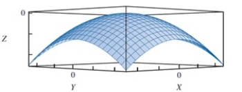
A)f(X, Y) = X2 + Y2
B)f(X, Y) = -X - Y
C)f(X, Y) = -X2 - Y2
D)f(X, Y) = Xsin(5ðX) + Ysin(5ðY)
A)f(X, Y) = X2 + Y2
B)f(X, Y) = -X - Y
C)f(X, Y) = -X2 - Y2
D)f(X, Y) = Xsin(5ðX) + Ysin(5ðY)
Question
Question
Question
Question
Question
Question
Question
Question
In reviewing the image below, the point (0, 0, 0) is a(n) __________ for the given concave function. 
A)local maximum
B)local minimum
C)convergence point
D)endpoint
A)local maximum
B)local minimum
C)convergence point
D)endpoint
Question
Question
Question
Question
Question
Using the graph below, the feasible region for the function represented in the graph is 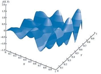
A)-1 £ X £ 1, -1 £ Y £ 1.
B)-1.5 £ X £ 1, 0 £ Y £ 8.
C)-1.5 £ X £ 2.0, -1.5 £ Y £ 2.0.
D)0 £ X £ 1, 0 £ Y £ 1.
A)-1 £ X £ 1, -1 £ Y £ 1.
B)-1.5 £ X £ 1, 0 £ Y £ 8.
C)-1.5 £ X £ 2.0, -1.5 £ Y £ 2.0.
D)0 £ X £ 1, 0 £ Y £ 1.
Question
Question
Using the graph below, which of the following is true of the above function? 
A)It has single local minimum.
B)It has multiple local optima.
C)It has single local maximum.
D)It has no maxima and minima.
A)It has single local minimum.
B)It has multiple local optima.
C)It has single local maximum.
D)It has no maxima and minima.
Question
Question
Question
Question
Question
Question
Which of the following conclusions can be drawn from the below figure using the Bass forecasting model? (Note: Bass forecasting model is given by: Ft = (p + q[Ct - 1 /m]) (m - Ct - 1),
Where m = the number of people estimated to eventually adopt the new product,
Ct - 1 = the number of people who have adopted the product through time t - 1,
Q = the coefficient of imitation, and
P = the coefficient of innovation.)![<strong>Which of the following conclusions can be drawn from the below figure using the Bass forecasting model? (Note: Bass forecasting model is given by: F<sub>t</sub> = (p + q[Ct<sub> - 1</sub> /m]) (m - Ct<sub> - 1</sub>), Where m = the number of people estimated to eventually adopt the new product, Ct<sub> - 1</sub> = the number of people who have adopted the product through time t - 1, Q = the coefficient of imitation, and P = the coefficient of innovation.) </strong> A)q < p B)q > p C)m < q D)p > m <div style=padding-top: 35px>](https://storage.examlex.com/TB2760/11eb0ecc_0968_4ed0_9431_3722522061cb_TB2760_00.jpg)
A)q < p
B)q > p
C)m < q
D)p > m
Where m = the number of people estimated to eventually adopt the new product,
Ct - 1 = the number of people who have adopted the product through time t - 1,
Q = the coefficient of imitation, and
P = the coefficient of innovation.)
A)q < p
B)q > p
C)m < q
D)p > m
Question
Question
Question
Question
Question
Question
Question
In reviewing the image below, what is the minimum value for this function? 
A)-8
B)0
C)-1
D)1
A)-8
B)0
C)-1
D)1
Question
Question
Using the graph given below, which of the following equations is most likely to yield the above curve? 
A)f(X, Y) = Xlog(2ðY) + Ylog(2ðX)
B)f(X, Y) = X - Y
C)f(X, Y) = -X2 - Y2
D)f(X, Y) = Xsin(5ðX) + Ysin(5ðY)
A)f(X, Y) = Xlog(2ðY) + Ylog(2ðX)
B)f(X, Y) = X - Y
C)f(X, Y) = -X2 - Y2
D)f(X, Y) = Xsin(5ðX) + Ysin(5ðY)
Question
Consider the following data on the returns from bonds. 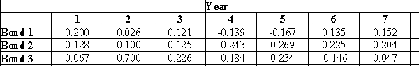 Develop and solve the Markowitz portfolio model using a required expected return of at least 15 percent. Assume that the 8 scenarios are equally likely to occur. Use this model to construct an efficient frontier by varying the expected return from 2 to 18 percent in increment of 2 percent and solving for the variance. Round all your answers to three decimal places.
Develop and solve the Markowitz portfolio model using a required expected return of at least 15 percent. Assume that the 8 scenarios are equally likely to occur. Use this model to construct an efficient frontier by varying the expected return from 2 to 18 percent in increment of 2 percent and solving for the variance. Round all your answers to three decimal places. Question
Question
Question
The exponential smoothing model is given by 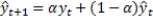 where
where 
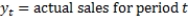

 This model is used to predict the future based on the past data values.
a. The observed values with the smoothing constant a = 0.45 are given in the below table. The third column of the table displays the forecast values obtained using the above model. The forecasted error is calculated in the fourth column, and the square of the forecast error and the sum of squared forecast errors are given in fifth column. Construct this table in your spreadsheet model using the formula above. (Hint: The first forecast value is same as the observed value.)
Alpha = 0.45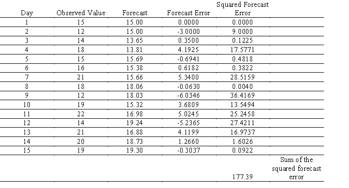
b. The value of á is often chosen by minimizing the sum of squared forecast errors. Use Excel Solver to find the value of á that minimizes the sum of squared forecast errors.
where This model is used to predict the future based on the past data values. a. The observed values with the smoothing constant a = 0.45 are given in the below table. The third column of the table displays the forecast values obtained using the above model. The forecasted error
is calculated in the fourth column, and the square of the forecast error and the sum of squared forecast errors are given in fifth column. Construct this table in your spreadsheet model using the formula above. (Hint: The first forecast value is same as the observed value.)Alpha = 0.45
b. The value of á is often chosen by minimizing the sum of squared forecast errors. Use Excel Solver to find the value of á that minimizes the sum of squared forecast errors.
Question
Consider the stock return data given below. 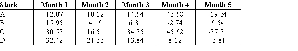 Develop and solve the Markowitz model that maximizes expected return subject to a maximum variance of 35. Use this model to construct an efficient frontier by varying the maximum allowable variance from 25 to 55 in increments of 5 and solving for the maximum return for each.
Develop and solve the Markowitz model that maximizes expected return subject to a maximum variance of 35. Use this model to construct an efficient frontier by varying the maximum allowable variance from 25 to 55 in increments of 5 and solving for the maximum return for each. Question
Consider the following data on the returns from bonds. 
a. Construct the Markowitz portfolio model using a required expected return of at least 15 percent. Assume that the 8 scenarios are equally likely to occur.
b. Solve the model using Excel Solver.
a. Construct the Markowitz portfolio model using a required expected return of at least 15 percent. Assume that the 8 scenarios are equally likely to occur.
b. Solve the model using Excel Solver.
Question
Consider the economic order quantity (EOQ) model for multiple products that are independent except for a budget restriction. The following model describes this situation
Let Dk = annual demand for product k
Ck = unit cost of product k
Sk = cost per order placed for product k
i = inventory carrying charge as a percentage of the cost per unit
B = the maximum amount of investment in goods
N = number of products
The decision variables are Qk, the amount of product k to order. The model is: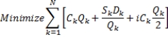 s.t.
s.t. 
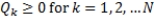
a. Set up a spreadsheet model and for the following data: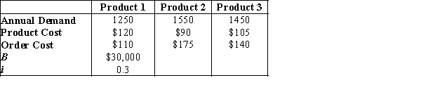
b. Solve the problem using Excel Solver. (Hint: For Solver to find a solution, you need to start with decision variable values that are greater than 0.)
Let Dk = annual demand for product k
Ck = unit cost of product k
Sk = cost per order placed for product k
i = inventory carrying charge as a percentage of the cost per unit
B = the maximum amount of investment in goods
N = number of products
The decision variables are Qk, the amount of product k to order. The model is:
s.t. a. Set up a spreadsheet model and for the following data:
b. Solve the problem using Excel Solver. (Hint: For Solver to find a solution, you need to start with decision variable values that are greater than 0.)
Question
Mark and his friends are planning for a holiday party. Data on longitude, latitude, and number of friends at each of the 10 locations are given below. Mark would like to identify the location for the holiday party such that it minimizes the demand-weighted distance, where demand is the number of friends at each location. Find the optimal location for the party. The distance between two cities can be approximated by the following formula.  where lat1 and long1 are the latitude and longitude of city 1, and lat2 and long2 are the latitude and longitude of city 2. (Hint: Notice that all longitude values given for this problem are negative. Make sure that you do not check the option for Make Unconstrained Variables Non-Negative in Solver.)
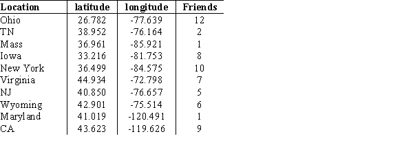
where lat1 and long1 are the latitude and longitude of city 1, and lat2 and long2 are the latitude and longitude of city 2. (Hint: Notice that all longitude values given for this problem are negative. Make sure that you do not check the option for Make Unconstrained Variables Non-Negative in Solver.) Question
Develop a model that minimizes semivariance for the data given below with a required return of 15 percent. Define a variable  for each scenario and let
  with
with  = 0. Then make the objective function: Min
  .
.  Solve the model you developed with a required expected return of at least 15 percent.
for each scenario and let with = 0. Then make the objective function: Min . Solve the model you developed with a required expected return of at least 15 percent. Question
Question
Consider the stock return data given below. 
a. Construct the Markowitz model that maximizes expected return subject to a maximum variance of 35.
a. Round all your answers to three decimal places.
b. Solve the model developed in part
a. Construct the Markowitz model that maximizes expected return subject to a maximum variance of 35.
a. Round all your answers to three decimal places.
b. Solve the model developed in part
Question
Jim must solve a nonlinear optimization problem where point A should be within a radius of 15 centimeters from each of the points B, C, D, E and F. The decision variables are defined as below.
X = horizontal coordinate of point A
Y = vertical coordinate of point A
The data on the distances is given below: Formulate and solve a model that minimizes the maximum distance from point A to each of the points B, C, D, E, and F. Round all your answers to three decimal places.
X = horizontal coordinate of point A
Y = vertical coordinate of point A
The data on the distances is given below:
Formulate and solve a model that minimizes the maximum distance from point A to each of the points B, C, D, E, and F. Round all your answers to three decimal places. Question
Jim must solve a nonlinear optimization problem where point A should be within a radius of 15 centimeters from each of the points B, C, D, E and F. The decision variables are defined as below.
X = horizontal coordinate of point A
Y = vertical coordinate of point A
The data on the distances is given below: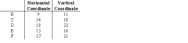 Formulate a model to find the optimal location of the point A.
X = horizontal coordinate of point A
Y = vertical coordinate of point A
The data on the distances is given below:
Formulate a model to find the optimal location of the point A. Question
Question

Unlock Deck
Sign up to unlock the cards in this deck!
Unlock Deck
Unlock Deck
1/55
Play
Full screen (f)
Deck 13: Nonlinear Optimization Models
1
A ____________ is the shadow price of a binding simple lower or upper bound on the decision variable.
A)reduced gradient
B)binding constraint
C)binary variable
D)local optimum
A)reduced gradient
B)binding constraint
C)binary variable
D)local optimum
reduced gradient
2
Which of the following functions yields the shape shown below?
A)f(X, Y) = X2 + Y2
B)f(X, Y) = Xsin(2ðY) + Ysin(2ðX)
C)f(X, Y) = -X2 - Y2
D)f(X, Y) = Xsin(5ðX) + Ysin(5ðY)
A)f(X, Y) = X2 + Y2
B)f(X, Y) = Xsin(2ðY) + Ysin(2ðX)
C)f(X, Y) = -X2 - Y2
D)f(X, Y) = Xsin(5ðX) + Ysin(5ðY)
f(X, Y) = X2 + Y2
3
A function that is bowl-shaped down is called a ___________ function.
A)concave
B)convex
C)conic
D)linear
A)concave
B)convex
C)conic
D)linear
concave
4
In a nonlinear optimization problem
A)the objective function is a nonlinear function of the constraints.
B)all the constraints are nonlinear only when the objective is to maximize the function of the decision variables.
C)at least one term in the objective function or a constraint is nonlinear.
D)both the objective function and the constraints must have all nonlinear terms.
Unlock Deck
Unlock for access to all 55 flashcards in this deck.
Unlock Deck
k this deck
5
A feasible solution is __________ if there are no other feasible points with a better objective function value in the entire feasible region.
A)infeasible
B)unbounded
C)nonlinear
D)a global optimum
A)infeasible
B)unbounded
C)nonlinear
D)a global optimum
Unlock Deck
Unlock for access to all 55 flashcards in this deck.
Unlock Deck
k this deck
6
The Lagrangian multiplier is the __________ for a constraint in a nonlinear problem.
A)shadow price
B)payoff value
C)reducing gradient
D)reduced cost
A)shadow price
B)payoff value
C)reducing gradient
D)reduced cost
Unlock Deck
Unlock for access to all 55 flashcards in this deck.
Unlock Deck
k this deck
7
A feasible solution is ____________ if there are no other feasible points with a smaller objective function value in the entire feasible region.
A)a global minimum
B)not a local maximum
C)not a local minimum
D)bowl-shaped
A)a global minimum
B)not a local maximum
C)not a local minimum
D)bowl-shaped
Unlock Deck
Unlock for access to all 55 flashcards in this deck.
Unlock Deck
k this deck
8
In a nonlinear problem, the rate of change of the objective function with respect to the right-hand side of a constraint is given by the
A)slope of the contour line.
B)local optimum.
C)Reducing gradient.
D)Lagrangian multiplier.
A)slope of the contour line.
B)local optimum.
C)Reducing gradient.
D)Lagrangian multiplier.
Unlock Deck
Unlock for access to all 55 flashcards in this deck.
Unlock Deck
k this deck
9
A function that is bowl-shaped up is called a(n) _________ function.
A)concave
B)optimal
C)convex
D)elliptical
A)concave
B)optimal
C)convex
D)elliptical
Unlock Deck
Unlock for access to all 55 flashcards in this deck.
Unlock Deck
k this deck
10
In reviewing the image below, which of the following functions is most likely to yield the above shape?
A)f(X, Y) = X2 + Y2
B)f(X, Y) = -X - Y
C)f(X, Y) = -X2 - Y2
D)f(X, Y) = Xsin(5ðX) + Ysin(5ðY)
A)f(X, Y) = X2 + Y2
B)f(X, Y) = -X - Y
C)f(X, Y) = -X2 - Y2
D)f(X, Y) = Xsin(5ðX) + Ysin(5ðY)
Unlock Deck
Unlock for access to all 55 flashcards in this deck.
Unlock Deck
k this deck
11
The reduced gradient is analogous to the ___________ for linear models.
A)binary variable
B)binding constraint
C)reduced cost
D)objective coefficient
A)binary variable
B)binding constraint
C)reduced cost
D)objective coefficient
Unlock Deck
Unlock for access to all 55 flashcards in this deck.
Unlock Deck
k this deck
12
If there are no other feasible points with a larger objective function value in the entire feasible region, a feasible solution is
A)an efficient frontier.
B)a global maximum.
C)not a local maximum.
D)a global minimum.
A)an efficient frontier.
B)a global maximum.
C)not a local maximum.
D)a global minimum.
Unlock Deck
Unlock for access to all 55 flashcards in this deck.
Unlock Deck
k this deck
13
A nonlinear function with term to the power of two is known as a
A)hyperbolic function.
B)quadratic function.
C)logarithmic function.
D)cubic function.
A)hyperbolic function.
B)quadratic function.
C)logarithmic function.
D)cubic function.
Unlock Deck
Unlock for access to all 55 flashcards in this deck.
Unlock Deck
k this deck
14
A global minimum
A)is also a local maximum.
B)need not be a local maximum, but vice versa is true.
C)is also a local minimum.
D)need not be local minimum, but vice versa is true.
A)is also a local maximum.
B)need not be a local maximum, but vice versa is true.
C)is also a local minimum.
D)need not be local minimum, but vice versa is true.
Unlock Deck
Unlock for access to all 55 flashcards in this deck.
Unlock Deck
k this deck
15
If all the squared terms in a quadratic function have a negative coefficient and there are no cross-product terms, then the function is a _____ function.
A)convex quadratic
B)nonlinear objective
C)concave quadratic
D)negative elliptical
A)convex quadratic
B)nonlinear objective
C)concave quadratic
D)negative elliptical
Unlock Deck
Unlock for access to all 55 flashcards in this deck.
Unlock Deck
k this deck
16
The ___________ of a solution is a mathematical concept that refers to the set of points within a relatively close proximity of the solution.
A)objective function contour
B)neighborhood
C)regression equation
D)Lagrangian multiplier
A)objective function contour
B)neighborhood
C)regression equation
D)Lagrangian multiplier
Unlock Deck
Unlock for access to all 55 flashcards in this deck.
Unlock Deck
k this deck
17
A feasible solution is a(n) ___________ if there are no other feasible solutions with a better objective function value in the immediate neighborhood.
A)efficient frontier
B)local optimum
C)global maximum
D)diverging function
A)efficient frontier
B)local optimum
C)global maximum
D)diverging function
Unlock Deck
Unlock for access to all 55 flashcards in this deck.
Unlock Deck
k this deck
18
In reviewing the image below, the point (0, 0, 0) is a(n) __________ for the given concave function.
A)local maximum
B)local minimum
C)convergence point
D)endpoint
A)local maximum
B)local minimum
C)convergence point
D)endpoint
Unlock Deck
Unlock for access to all 55 flashcards in this deck.
Unlock Deck
k this deck
19
If there are no other feasible solutions with a larger objective function value in the immediate neighborhood, then the feasible solution is known as
A)a global maximum.
B)infeasible.
C)a nonlinear solution.
D)a local maximum.
A)a global maximum.
B)infeasible.
C)a nonlinear solution.
D)a local maximum.
Unlock Deck
Unlock for access to all 55 flashcards in this deck.
Unlock Deck
k this deck
20
A feasible solution is a local minimum if there are no other feasible solutions with a
A)smaller objective function value in the immediate neighborhood.
B)same objective function value in the immediate neighborhood.
C)set of points defining the minimum possible risk in the entire feasible region.
D)same objective function value in the entire feasible region.
A)smaller objective function value in the immediate neighborhood.
B)same objective function value in the immediate neighborhood.
C)set of points defining the minimum possible risk in the entire feasible region.
D)same objective function value in the entire feasible region.
Unlock Deck
Unlock for access to all 55 flashcards in this deck.
Unlock Deck
k this deck
21
Excel Solver's __________ is based on a method that searches for an optimal solution by iteratively adjusting a population of candidate solutions.
A)Evolutionary Solver
B)Goal Seeker
C)Simplex LP
D)GRG Nonlinear
A)Evolutionary Solver
B)Goal Seeker
C)Simplex LP
D)GRG Nonlinear
Unlock Deck
Unlock for access to all 55 flashcards in this deck.
Unlock Deck
k this deck
22
The __________forecasting model uses nonlinear optimization to forecast the adoption of innovative and new technologies in the marketplace.
A)Hauck
B)LMS
C)Markowitz
D)Bass
A)Hauck
B)LMS
C)Markowitz
D)Bass
Unlock Deck
Unlock for access to all 55 flashcards in this deck.
Unlock Deck
k this deck
23
Using the graph below, the feasible region for the function represented in the graph is
A)-1 £ X £ 1, -1 £ Y £ 1.
B)-1.5 £ X £ 1, 0 £ Y £ 8.
C)-1.5 £ X £ 2.0, -1.5 £ Y £ 2.0.
D)0 £ X £ 1, 0 £ Y £ 1.
A)-1 £ X £ 1, -1 £ Y £ 1.
B)-1.5 £ X £ 1, 0 £ Y £ 8.
C)-1.5 £ X £ 2.0, -1.5 £ Y £ 2.0.
D)0 £ X £ 1, 0 £ Y £ 1.
Unlock Deck
Unlock for access to all 55 flashcards in this deck.
Unlock Deck
k this deck
24
The measure of risk most often associated with the Markowitz portfolio model is the
A)expected return of the portfolio.
B)annual interest on the portfolio.
C)variance of the portfolio's return.
D)number of investments listed in the portfolio.
A)expected return of the portfolio.
B)annual interest on the portfolio.
C)variance of the portfolio's return.
D)number of investments listed in the portfolio.
Unlock Deck
Unlock for access to all 55 flashcards in this deck.
Unlock Deck
k this deck
25
Using the graph below, which of the following is true of the above function?
A)It has single local minimum.
B)It has multiple local optima.
C)It has single local maximum.
D)It has no maxima and minima.
A)It has single local minimum.
B)It has multiple local optima.
C)It has single local maximum.
D)It has no maxima and minima.
Unlock Deck
Unlock for access to all 55 flashcards in this deck.
Unlock Deck
k this deck
26
In the Bass forecasting model, the ___________measures the likelihood of adoption, assuming no influence from someone who has already purchased (adopted) the product.
A)coefficient of correlation
B)coefficient of imitation
C)coefficient of independence
D)coefficient of innovation
A)coefficient of correlation
B)coefficient of imitation
C)coefficient of independence
D)coefficient of innovation
Unlock Deck
Unlock for access to all 55 flashcards in this deck.
Unlock Deck
k this deck
27
In the Bass forecasting model, the __________ measures the likelihood of adoption due to a potential adopter being influenced by someone who has already adopted the product.
A)coefficient of innovation
B)coefficient of imitation
C)coefficient of regression
D)coefficient of the objective function
A)coefficient of innovation
B)coefficient of imitation
C)coefficient of regression
D)coefficient of the objective function
Unlock Deck
Unlock for access to all 55 flashcards in this deck.
Unlock Deck
k this deck
28
Which of the following is a second way of formulating the Markowitz model?
A)Maximizing the expected return of the portfolio subject to a constraint on variance
B)Minimizing the expected return of the portfolio subject to a constraint on variance.
C)Maximizing the variance of the portfolio subject to a constraint on the expected return of the portfolio
D)Maximizing the variance of the portfolio with no constraint needed for the expected return of the portfolio
Unlock Deck
Unlock for access to all 55 flashcards in this deck.
Unlock Deck
k this deck
29
If the portfolio variance were equal to zero, the amount of risk would be
A)unity.
B)a positive number greater than 1.
C)negative always.
D)zero.
A)unity.
B)a positive number greater than 1.
C)negative always.
D)zero.
Unlock Deck
Unlock for access to all 55 flashcards in this deck.
Unlock Deck
k this deck
30
The __________ option in Excel Solver is helpful when the solution to a problem appears to depend on the starting values for the decision variables.
A)Restart
B)Convergence
C)Derivatives
D)Multistart
A)Restart
B)Convergence
C)Derivatives
D)Multistart
Unlock Deck
Unlock for access to all 55 flashcards in this deck.
Unlock Deck
k this deck
31
Which of the following conclusions can be drawn from the below figure using the Bass forecasting model? (Note: Bass forecasting model is given by: Ft = (p + q[Ct - 1 /m]) (m - Ct - 1),
Where m = the number of people estimated to eventually adopt the new product,
Ct - 1 = the number of people who have adopted the product through time t - 1,
Q = the coefficient of imitation, and
P = the coefficient of innovation.)
A)q < p
B)q > p
C)m < q
D)p > m
Where m = the number of people estimated to eventually adopt the new product,
Ct - 1 = the number of people who have adopted the product through time t - 1,
Q = the coefficient of imitation, and
P = the coefficient of innovation.)
A)q < p
B)q > p
C)m < q
D)p > m
Unlock Deck
Unlock for access to all 55 flashcards in this deck.
Unlock Deck
k this deck
32
A(n) __________ is a set of points defining the minimum possible risk for a set of return values.
A)contour
B)efficient frontier
C)unity constraint
D)reduced gradient
A)contour
B)efficient frontier
C)unity constraint
D)reduced gradient
Unlock Deck
Unlock for access to all 55 flashcards in this deck.
Unlock Deck
k this deck
33
The portfolio variance is the
A)sum of the squares of the deviations from the mean value under each scenario.
B)average of the sum of the squares of the deviations from the mean value under each investment scenario.
C)average of the product of the squares of the deviations from the mean value under each scenario.
D)average of the sum of the deviations from the mean value under each investment scenario.
Unlock Deck
Unlock for access to all 55 flashcards in this deck.
Unlock Deck
k this deck
34
A portfolio optimization model used to construct a portfolio that minimizes risk subject to a constraint requiring a minimum level of return is known as
A)capital budgeting pricing model.
B)market share optimization model.
C)Hauck maximum variance portfolio model.
D)Markowitz mean-variance portfolio model.
A)capital budgeting pricing model.
B)market share optimization model.
C)Hauck maximum variance portfolio model.
D)Markowitz mean-variance portfolio model.
Unlock Deck
Unlock for access to all 55 flashcards in this deck.
Unlock Deck
k this deck
35
One of the ways to use the Bass forecasting model is to wait until several periods of data for the problem under consideration are available. This is known as the ___________ approach.
A)branch-and-bound
B)cutting plane
C)rolling-horizon
D)sensible-period
A)branch-and-bound
B)cutting plane
C)rolling-horizon
D)sensible-period
Unlock Deck
Unlock for access to all 55 flashcards in this deck.
Unlock Deck
k this deck
36
Solving nonlinear problems with local optimal solutions is performed using _____________, in Excel Solver, which is based on more classical optimization techniques.
A)Goal Seeker
B)Linear Regression
C)GRG Nonlinear
D)Simplex LP
A)Goal Seeker
B)Linear Regression
C)GRG Nonlinear
D)Simplex LP
Unlock Deck
Unlock for access to all 55 flashcards in this deck.
Unlock Deck
k this deck
37
In the Bass forecasting model, parameter m
A)measures the likelihood of adoption due to a potential adopter being influenced by someone who has already adopted the product.
B)measures the likelihood of adoption, assuming no influence from someone who has already adopted the product.
C)refers to the number of people estimated to eventually adopt the new product.
D)refers to the number of people who have already adopted the new product.
Unlock Deck
Unlock for access to all 55 flashcards in this deck.
Unlock Deck
k this deck
38
In reviewing the image below, what is the minimum value for this function?
A)-8
B)0
C)-1
D)1
A)-8
B)0
C)-1
D)1
Unlock Deck
Unlock for access to all 55 flashcards in this deck.
Unlock Deck
k this deck
39
One of the ways to formulate the Markowitz model is to
A)maximize the variance of the portfolio subject to a constraint on the expected return of the portfolio.
B)minimize the expected return of the portfolio subject to a constraint on variance.
C)minimize the variance of the portfolio subject to a constraint on the expected return of the portfolio.
D)minimize the expected return of the portfolio with no constraint on variance.
Unlock Deck
Unlock for access to all 55 flashcards in this deck.
Unlock Deck
k this deck
40
Using the graph given below, which of the following equations is most likely to yield the above curve?
A)f(X, Y) = Xlog(2ðY) + Ylog(2ðX)
B)f(X, Y) = X - Y
C)f(X, Y) = -X2 - Y2
D)f(X, Y) = Xsin(5ðX) + Ysin(5ðY)
A)f(X, Y) = Xlog(2ðY) + Ylog(2ðX)
B)f(X, Y) = X - Y
C)f(X, Y) = -X2 - Y2
D)f(X, Y) = Xsin(5ðX) + Ysin(5ðY)
Unlock Deck
Unlock for access to all 55 flashcards in this deck.
Unlock Deck
k this deck
41
Consider the following data on the returns from bonds. Develop and solve the Markowitz portfolio model using a required expected return of at least 15 percent. Assume that the 8 scenarios are equally likely to occur. Use this model to construct an efficient frontier by varying the expected return from 2 to 18 percent in increment of 2 percent and solving for the variance. Round all your answers to three decimal places.
Develop and solve the Markowitz portfolio model using a required expected return of at least 15 percent. Assume that the 8 scenarios are equally likely to occur. Use this model to construct an efficient frontier by varying the expected return from 2 to 18 percent in increment of 2 percent and solving for the variance. Round all your answers to three decimal places. Unlock Deck
Unlock for access to all 55 flashcards in this deck.
Unlock Deck
k this deck
42
A Steel Manufacturing company has two production facilities that manufacture Dishwashers. Production costs at the two facilities differ because of varying labor costs, local property taxes, type of material used, volume, and so on. For Plant A, the weekly costs for producing a number of units of Dishwashers is expressed as a function
TCA(X) = X2 - 2X + 12000
where X is the weekly production volume and TCA(X) is the weekly cost for Plant A. Plant B's weekly production costs are given by
TCB(Y) = Y2 + 8Y + 10000
where Y is the weekly production volume and TCB(Y) is the weekly cost for Plant B. The manufacturer would like to produce 50 dishwashers per week at the lowest possible cost.
a. Formulate a mathematical model that can be used to determine the optimal number of dishwashers to produce each week at each facility.
b. Solve the optimization model to determine the optimal number of dishwashers to produce at each facility.
Unlock Deck
Unlock for access to all 55 flashcards in this deck.
Unlock Deck
k this deck
43
Roger is willing to promote and sell two types of smart watches, X and Y, at his outlet. The demand for these two watches are as follows.
DX = -0.45PX + 0.34PY + 242
DY = 0.2PX - 0.58PY+ 282
where, DX is the demand for watch X, PX is the selling price of watch X, DY is the demand for watch Y, and PY is the selling price of watch Y.
Rogers wishes to determine the selling price that maximizes revenue for these two products. Develop the revenue function for these two models, and find the revenue maximizing prices.
Unlock Deck
Unlock for access to all 55 flashcards in this deck.
Unlock Deck
k this deck
44
The exponential smoothing model is given by where This model is used to predict the future based on the past data values.
a. The observed values with the smoothing constant a = 0.45 are given in the below table. The third column of the table displays the forecast values obtained using the above model. The forecasted error is calculated in the fourth column, and the square of the forecast error and the sum of squared forecast errors are given in fifth column. Construct this table in your spreadsheet model using the formula above. (Hint: The first forecast value is same as the observed value.)
Alpha = 0.45
b. The value of á is often chosen by minimizing the sum of squared forecast errors. Use Excel Solver to find the value of á that minimizes the sum of squared forecast errors.
where This model is used to predict the future based on the past data values. a. The observed values with the smoothing constant a = 0.45 are given in the below table. The third column of the table displays the forecast values obtained using the above model. The forecasted error
is calculated in the fourth column, and the square of the forecast error and the sum of squared forecast errors are given in fifth column. Construct this table in your spreadsheet model using the formula above. (Hint: The first forecast value is same as the observed value.)Alpha = 0.45
b. The value of á is often chosen by minimizing the sum of squared forecast errors. Use Excel Solver to find the value of á that minimizes the sum of squared forecast errors.
Unlock Deck
Unlock for access to all 55 flashcards in this deck.
Unlock Deck
k this deck
45
Consider the stock return data given below. Develop and solve the Markowitz model that maximizes expected return subject to a maximum variance of 35. Use this model to construct an efficient frontier by varying the maximum allowable variance from 25 to 55 in increments of 5 and solving for the maximum return for each.
Develop and solve the Markowitz model that maximizes expected return subject to a maximum variance of 35. Use this model to construct an efficient frontier by varying the maximum allowable variance from 25 to 55 in increments of 5 and solving for the maximum return for each. Unlock Deck
Unlock for access to all 55 flashcards in this deck.
Unlock Deck
k this deck
46
Consider the following data on the returns from bonds.
a. Construct the Markowitz portfolio model using a required expected return of at least 15 percent. Assume that the 8 scenarios are equally likely to occur.
b. Solve the model using Excel Solver.
a. Construct the Markowitz portfolio model using a required expected return of at least 15 percent. Assume that the 8 scenarios are equally likely to occur.
b. Solve the model using Excel Solver.
Unlock Deck
Unlock for access to all 55 flashcards in this deck.
Unlock Deck
k this deck
47
Consider the economic order quantity (EOQ) model for multiple products that are independent except for a budget restriction. The following model describes this situation
Let Dk = annual demand for product k
Ck = unit cost of product k
Sk = cost per order placed for product k
i = inventory carrying charge as a percentage of the cost per unit
B = the maximum amount of investment in goods
N = number of products
The decision variables are Qk, the amount of product k to order. The model is: s.t.
a. Set up a spreadsheet model and for the following data:
b. Solve the problem using Excel Solver. (Hint: For Solver to find a solution, you need to start with decision variable values that are greater than 0.)
Let Dk = annual demand for product k
Ck = unit cost of product k
Sk = cost per order placed for product k
i = inventory carrying charge as a percentage of the cost per unit
B = the maximum amount of investment in goods
N = number of products
The decision variables are Qk, the amount of product k to order. The model is:
s.t. a. Set up a spreadsheet model and for the following data:
b. Solve the problem using Excel Solver. (Hint: For Solver to find a solution, you need to start with decision variable values that are greater than 0.)
Unlock Deck
Unlock for access to all 55 flashcards in this deck.
Unlock Deck
k this deck
48
Mark and his friends are planning for a holiday party. Data on longitude, latitude, and number of friends at each of the 10 locations are given below. Mark would like to identify the location for the holiday party such that it minimizes the demand-weighted distance, where demand is the number of friends at each location. Find the optimal location for the party. The distance between two cities can be approximated by the following formula. where lat1 and long1 are the latitude and longitude of city 1, and lat2 and long2 are the latitude and longitude of city 2. (Hint: Notice that all longitude values given for this problem are negative. Make sure that you do not check the option for Make Unconstrained Variables Non-Negative in Solver.)
where lat1 and long1 are the latitude and longitude of city 1, and lat2 and long2 are the latitude and longitude of city 2. (Hint: Notice that all longitude values given for this problem are negative. Make sure that you do not check the option for Make Unconstrained Variables Non-Negative in Solver.) Unlock Deck
Unlock for access to all 55 flashcards in this deck.
Unlock Deck
k this deck
49
Develop a model that minimizes semivariance for the data given below with a required return of 15 percent. Define a variable for each scenario and let with = 0. Then make the objective function: Min . Solve the model you developed with a required expected return of at least 15 percent.
for each scenario and let with = 0. Then make the objective function: Min . Solve the model you developed with a required expected return of at least 15 percent. Unlock Deck
Unlock for access to all 55 flashcards in this deck.
Unlock Deck
k this deck
50
Jeff is willing to invest $5000 in buying shares and bonds of a company to gain maximum returns. From his past experience, he estimates the relationship between returns and investments made in this company to be:
R = -2S2 - 9B2 - 4SB + 20S + 30B.
where,
R = total returns in thousands of dollars
S = thousands of dollars spent on Shares
B = thousands of dollars spent on Bond
Jeff would like to develop a strategy that will lead to maximum return subject to the restriction provided on amount available for investment.
a. What is the value of return if $3,000 is invested in shares and $2,000 is invested bonds of the company?
b. Formulate an optimization problem that can be solved to maximize the returns subject to investing no more than $5,000 on both share and bonds.
c. Determine the optimal amount to invest in shares and bonds of the company. How much return will Jeff gain? Round all your answers to two decimal places.
Unlock Deck
Unlock for access to all 55 flashcards in this deck.
Unlock Deck
k this deck
51
Consider the stock return data given below.
a. Construct the Markowitz model that maximizes expected return subject to a maximum variance of 35.
a. Round all your answers to three decimal places.
b. Solve the model developed in part
a. Construct the Markowitz model that maximizes expected return subject to a maximum variance of 35.
a. Round all your answers to three decimal places.
b. Solve the model developed in part
Unlock Deck
Unlock for access to all 55 flashcards in this deck.
Unlock Deck
k this deck
52
Jim must solve a nonlinear optimization problem where point A should be within a radius of 15 centimeters from each of the points B, C, D, E and F. The decision variables are defined as below.
X = horizontal coordinate of point A
Y = vertical coordinate of point A
The data on the distances is given below: Formulate and solve a model that minimizes the maximum distance from point A to each of the points B, C, D, E, and F. Round all your answers to three decimal places.
X = horizontal coordinate of point A
Y = vertical coordinate of point A
The data on the distances is given below:
Formulate and solve a model that minimizes the maximum distance from point A to each of the points B, C, D, E, and F. Round all your answers to three decimal places. Unlock Deck
Unlock for access to all 55 flashcards in this deck.
Unlock Deck
k this deck
53
Jim must solve a nonlinear optimization problem where point A should be within a radius of 15 centimeters from each of the points B, C, D, E and F. The decision variables are defined as below.
X = horizontal coordinate of point A
Y = vertical coordinate of point A
The data on the distances is given below: Formulate a model to find the optimal location of the point A.
X = horizontal coordinate of point A
Y = vertical coordinate of point A
The data on the distances is given below:
Formulate a model to find the optimal location of the point A. Unlock Deck
Unlock for access to all 55 flashcards in this deck.
Unlock Deck
k this deck
54
Gatson manufacturing company is willing to promote 2 types of tires: Economy tire and Premium tire. These two tires are independent of each other in terms of demand, cost, price, etc. An analytics team of this company has estimated the profit functions for both the tires as
Monthly profit for Economy tire = 49.2415 IN(XA) + 180.414
Monthly profit for Premium tire = 84.344 IN(XB) - 150.112
where XA and XB are the advertising amount allocated to Economy tire and Premium tire, respectively, and IN is the natural logarithm function. The advertising budget is $200,000, and management has dictated that at least $20,000 must be allocated to each of the two tires.
(Hint: To compute a natural logarithm for the value X in Excel, use the formula = IN(X). For Solver to find an answer, you also need to start with decision variable values greater than 0 in this problem.)
Develop and solve an optimization model that will prescribe how the company should allocate its marketing budget to maximize profit.
Unlock Deck
Unlock for access to all 55 flashcards in this deck.
Unlock Deck
k this deck
55
An Electrical Company has two manufacturing plants. The cost in dollars of producing an Amplifier at each of the two plants is given below. The cost of producing Q1 Amplifiers at first plant is:
65Q1 + 4Q12+ 90
and the cost of producing Q2 Amplifiers at the second plant is
20Q2 + 2Q22+ 120
The company needs to manufacture at least 60 Amplifiers to meet the received orders. How many Amplifiers should be produced at each of the plant to minimize the total production cost? Round the answers to two decimal places and the total cost to the nearest dollar value.
Unlock Deck
Unlock for access to all 55 flashcards in this deck.
Unlock Deck
k this deck
Unlock Deck
Unlock for access to all 55 flashcards in this deck.


