Deck 8: Cost
Full screen (f)
Question
A firm has monthly production function
 where L is worker hours per month and K is square feet of manufacturing space.
a. If the hourly wage rate is $50 and manufacturing space costs $25 per square foot per month, what is the firm's least-cost input combination for producing 100 units
b. Graph its output expansion path.
c. What is its cost function
where L is worker hours per month and K is square feet of manufacturing space.a. If the hourly wage rate is $50 and manufacturing space costs $25 per square foot per month, what is the firm's least-cost input combination for producing 100 units
b. Graph its output expansion path.
c. What is its cost function
Question
Question
Suppose Noah and Naomi's short-run weekly production function is Q = F(L) = 2
 and the wage rate is $12 an hour. Suppose also that the sunk cost (for their fixed garage-space input) is $500 per week. What is their short-run weekly cost function Graph this cost function.
and the wage rate is $12 an hour. Suppose also that the sunk cost (for their fixed garage-space input) is $500 per week. What is their short-run weekly cost function Graph this cost function. Question
Question
Question
Question
Suppose a unit of capital instead costs Hannah and Sam $1,000 per week. Their production function and wage rate are the same as in Worked-Out Problem 8.2. What is their least-cost input combination for remodeling 100 square feet a week What is their total cost
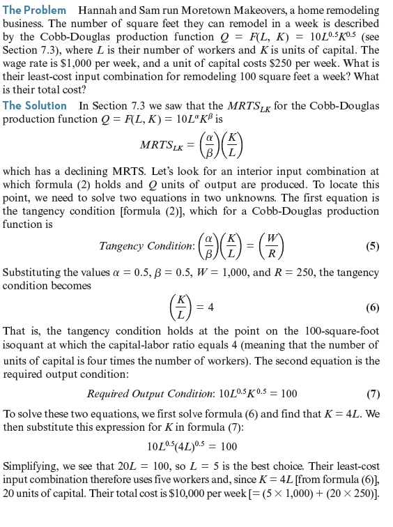
Worked-Out Problem 8.2

Worked-Out Problem 8.2
Question
Question
Question
Question
Question
Question
Question
Question
Question
Question
Question
Question
Question
Question
Question
Suppose that Hannah and Sam have the same production function as in Worked-Out Problem 8.2: Q = F ( L , K ) = 10 L 0.5 K 0.5. The wage rate is $1,000 per week and a unit of capital costs $250 per week. What is their least-cost input combination if they need to remodel 200 square feet per week What is their total cost
Worked-Out Problem 8.2

Worked-Out Problem 8.2
Question
A firm's technology for producing its output from labor ( L ) and capital (K) is
 . The wage is $2 per unit of labor and the cost of capital is $5 per unit of capital.
a. Does the firm's technology have a declining MRTS LK
b. What is the firm's cost function if both inputs are variable
c. Does the firm have economies of scale, diseconomies of scale, or neither
d. Suppose that the firm is initially producing 30 units of output. What is its cost function in the short run (when capital is fixed) Graph the long-run cost function and this short-run cost function in the same figure, labeling clearly all the important features such as where they each hit the vertical axis and any places they touch.
. The wage is $2 per unit of labor and the cost of capital is $5 per unit of capital.a. Does the firm's technology have a declining MRTS LK
b. What is the firm's cost function if both inputs are variable
c. Does the firm have economies of scale, diseconomies of scale, or neither
d. Suppose that the firm is initially producing 30 units of output. What is its cost function in the short run (when capital is fixed) Graph the long-run cost function and this short-run cost function in the same figure, labeling clearly all the important features such as where they each hit the vertical axis and any places they touch.
Question
Question
Suppose that Hannah and Sam have the same production function as in Worked-Out Problem 8.2: Q = F ( L , K ) = 10 L 0.5 K 0.5. The wage rate is $1,000 per week and a unit of capital costs $4,000 per week. Graph their output expansion path. What is their cost function
Worked-Out Problem 8.2

Worked-Out Problem 8.2
Question
(Calculus version below.) A firm has a monthly production function
 , where L is hours of labor per month and K is square feet of manufacturing space. The marginal product of labor is MP L = 1, while the marginal product of capital is
 .
.
a. If the hourly wage is $50 and manufacturing space costs $25 per square foot per month, what is the firm's least-cost input combination for producing 100 units
b. Graph its output expansion path.
c. What is its cost function
, where L is hours of labor per month and K is square feet of manufacturing space. The marginal product of labor is MP L = 1, while the marginal product of capital is .a. If the hourly wage is $50 and manufacturing space costs $25 per square foot per month, what is the firm's least-cost input combination for producing 100 units
b. Graph its output expansion path.
c. What is its cost function
Question
Question
Question
Question
(Suppose that Dan's Pizza Company in Worked-Out Problem 8.6 (page 271) instead has an avoidable fixed cost of $720 per day. What is his efficient scale of production What is his minimum average cost
Worked-Out Problem 8.6
The Problem Consider again Hannah and Sam's remodeling business described in Worked-Out Problems 8.2 and 8.3 (pages 254 and 256). They have a Cobb-Douglas production function Q = F ( L , K ) = 10 L 0.5 K 0.5 , and face a wage rate of $1, 000 per week, and a capital price of $250 per week per unit. Suppose that they are initially remodeling 100 square feet per week using the least-cost input combination for producing that output level. What are their short-run and long-run cost functions if their capital is fixed in the short run, but variable in the long run
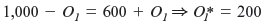
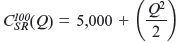
The Solution The solution to Worked-Out Problem 8.2 tells us that they initially use 20 units of capital. So, if their capital is fixed at 20 units, to remodel Q square feet Hannah and Sam need the amount of labor L that solves the formula

which means that L = ( Q 2 /2,000). So, their short-run cost function is

Or equivalently,

In contrast, the solution to Worked-Out Problem 8.3 tells us that Hannah and Sam's long-run cost function is
C LR ( Q ) = 100 Q
Observe, though, that their short-run and long-run costs are equal when Q = 100
 , just as our discussion indicated they must be.
Worked-Out Problem 8.2

Worked-Out Problem 8.3

Worked-Out Problem 8.6
The Problem Consider again Hannah and Sam's remodeling business described in Worked-Out Problems 8.2 and 8.3 (pages 254 and 256). They have a Cobb-Douglas production function Q = F ( L , K ) = 10 L 0.5 K 0.5 , and face a wage rate of $1, 000 per week, and a capital price of $250 per week per unit. Suppose that they are initially remodeling 100 square feet per week using the least-cost input combination for producing that output level. What are their short-run and long-run cost functions if their capital is fixed in the short run, but variable in the long run
The Solution The solution to Worked-Out Problem 8.2 tells us that they initially use 20 units of capital. So, if their capital is fixed at 20 units, to remodel Q square feet Hannah and Sam need the amount of labor L that solves the formula
which means that L = ( Q 2 /2,000). So, their short-run cost function is
Or equivalently,
In contrast, the solution to Worked-Out Problem 8.3 tells us that Hannah and Sam's long-run cost function is
C LR ( Q ) = 100 Q
Observe, though, that their short-run and long-run costs are equal when Q = 100
, just as our discussion indicated they must be.Worked-Out Problem 8.2
Worked-Out Problem 8.3
Question
Question
(Suppose that in Worked-Out Problem 8.4 (page 261), the cost function at plant 2 was C 2 ( Q 2 ) = 650 Q 2 + 2( Q 2 ) 2 , and marginal cost at that plant was MC 2 = 650 + 4 Q 2. What would be the best assignment of output between the two plants
Worked-Out Problem 8.4
The Problem Suppose Noah and Naomi have just acquired a second garden bench production plant. Production costs are C 1 ( Q 1 ) = 3( Q 1 ) 2 at plant 1 and C 2 (Q 2 ) = 2( Q 2 ) 2 at plant 2, where Q 1 and Q 2 are the number of benches produced at each plant per week. The corresponding marginal costs at the two plants are MC 1 = 6 Q 1 and MC 2 = 4 Q 2. If Noah and Naomi plan to produce 100 benches per week and want to do it as economically as possible, how many benches should they produce at each plant

The Solution The basic principle behind the solution to this problem is similar to that in Worked-Out Problem 7.1 (page 216). With a least-cost plan that assigns a positive amount of output to each plant, marginal cost must be the same at both plants. If that were not true, the total cost could be lowered by reassigning a little bit of output from the plant with the higher marginal cost to the plant with the lower marginal cost.
Noah and Naomi need to divide production between the two plants so that their marginal costs are equal. Doing so means choosing Q 1 and Q 2 so that MC 1 = MC 2. Since total output equals 100, we know that Q 2 = 100 Q 1 , so we can express the marginal cost in plant 2 as a function of the amount of output produced in plant 1: MC 2 = 4(100 - Q 1 ). We can then find the output assignment that equates marginal costs in the two plants by solving the formula
6 Q 1 = 4(100 - Q 1 )The solution is Q 1 = 40. Noah and Naomi should produce 40 garden benches a week in plant 1 and 60 garden benches a week in plant 2. Their total production costs will then be
C = 3(40) 2 + 2(60) 2 = $12,000
Worked-Out Problem 7.1
The Problem John, April, and Tristan own JATjuice, a firm that produces freshly squeezed orange juice. Oranges are their only variable input. They have two production facilities. Suppose the marginal product of oranges in plant 1 is
 , where O 1 is the number of crates of oranges allocated to plant 1. The marginal product of oranges in plant 2 is
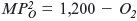 , where O 2 is the number of crates of oranges assigned to plant 2. Suppose that John, April, and Tristan have a total of 600 crates of oranges. What is the best assignment of oranges to the two plants

The Solution Start by writing the marginal product in plant 2asa function of the number of crates of oranges assigned to plant 1, O 1 :
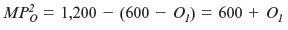
Now find the level of O 1 that equates the marginal product of oranges in the two plants. We can do so with algebra by setting
 and solving:
John, April, and Tristan should assign 200 crates to plant 1 and the rest (400) to plant 2.
Worked-Out Problem 8.4
The Problem Suppose Noah and Naomi have just acquired a second garden bench production plant. Production costs are C 1 ( Q 1 ) = 3( Q 1 ) 2 at plant 1 and C 2 (Q 2 ) = 2( Q 2 ) 2 at plant 2, where Q 1 and Q 2 are the number of benches produced at each plant per week. The corresponding marginal costs at the two plants are MC 1 = 6 Q 1 and MC 2 = 4 Q 2. If Noah and Naomi plan to produce 100 benches per week and want to do it as economically as possible, how many benches should they produce at each plant
The Solution The basic principle behind the solution to this problem is similar to that in Worked-Out Problem 7.1 (page 216). With a least-cost plan that assigns a positive amount of output to each plant, marginal cost must be the same at both plants. If that were not true, the total cost could be lowered by reassigning a little bit of output from the plant with the higher marginal cost to the plant with the lower marginal cost.
Noah and Naomi need to divide production between the two plants so that their marginal costs are equal. Doing so means choosing Q 1 and Q 2 so that MC 1 = MC 2. Since total output equals 100, we know that Q 2 = 100 Q 1 , so we can express the marginal cost in plant 2 as a function of the amount of output produced in plant 1: MC 2 = 4(100 - Q 1 ). We can then find the output assignment that equates marginal costs in the two plants by solving the formula
6 Q 1 = 4(100 - Q 1 )The solution is Q 1 = 40. Noah and Naomi should produce 40 garden benches a week in plant 1 and 60 garden benches a week in plant 2. Their total production costs will then be
C = 3(40) 2 + 2(60) 2 = $12,000
Worked-Out Problem 7.1
The Problem John, April, and Tristan own JATjuice, a firm that produces freshly squeezed orange juice. Oranges are their only variable input. They have two production facilities. Suppose the marginal product of oranges in plant 1 is
, where O 1 is the number of crates of oranges allocated to plant 1. The marginal product of oranges in plant 2 is , where O 2 is the number of crates of oranges assigned to plant 2. Suppose that John, April, and Tristan have a total of 600 crates of oranges. What is the best assignment of oranges to the two plants The Solution Start by writing the marginal product in plant 2asa function of the number of crates of oranges assigned to plant 1, O 1 :
Now find the level of O 1 that equates the marginal product of oranges in the two plants. We can do so with algebra by setting
and solving: John, April, and Tristan should assign 200 crates to plant 1 and the rest (400) to plant 2.
Question
Question
(Consider again Worked-Out Problem 8.6 (page 271) but assume that Hannah and Sam are initially remodeling 200 square feet per week. What are their short-run and long-run cost functions if capital is fixed in the short run, but variable in the long run
Worked-Out Problem 8.6
The Problem Consider again Hannah and Sam's remodeling business described in Worked-Out Problems 8.2 and 8.3 (pages 254 and 256). They have a Cobb-Douglas production function Q = F ( L , K ) = 10 L 0.5 K 0.5 , and face a wage rate of $1, 000 per week, and a capital price of $250 per week per unit. Suppose that they are initially remodeling 100 square feet per week using the least-cost input combination for producing that output level. What are their short-run and long-run cost functions if their capital is fixed in the short run, but variable in the long run
The Solution The solution to Worked-Out Problem 8.2 tells us that they initially use 20 units of capital. So, if their capital is fixed at 20 units, to remodel Q square feet Hannah and Sam need the amount of labor L that solves the formula

which means that L = ( Q 2 /2,000). So, their short-run cost function is
Or equivalently,

In contrast, the solution to Worked-Out Problem 8.3 tells us that Hannah and Sam's long-run cost function is
C LR ( Q ) = 100 Q
Observe, though, that their short-run and long-run costs are equal when Q = 100
 , just as our discussion indicated they must be.
Worked-Out Problem 8.2

Worked-Out Problem 8.3
Worked-Out Problem 8.6
The Problem Consider again Hannah and Sam's remodeling business described in Worked-Out Problems 8.2 and 8.3 (pages 254 and 256). They have a Cobb-Douglas production function Q = F ( L , K ) = 10 L 0.5 K 0.5 , and face a wage rate of $1, 000 per week, and a capital price of $250 per week per unit. Suppose that they are initially remodeling 100 square feet per week using the least-cost input combination for producing that output level. What are their short-run and long-run cost functions if their capital is fixed in the short run, but variable in the long run
The Solution The solution to Worked-Out Problem 8.2 tells us that they initially use 20 units of capital. So, if their capital is fixed at 20 units, to remodel Q square feet Hannah and Sam need the amount of labor L that solves the formula
which means that L = ( Q 2 /2,000). So, their short-run cost function is
Or equivalently,
In contrast, the solution to Worked-Out Problem 8.3 tells us that Hannah and Sam's long-run cost function is
C LR ( Q ) = 100 Q
Observe, though, that their short-run and long-run costs are equal when Q = 100
, just as our discussion indicated they must be.Worked-Out Problem 8.2
Worked-Out Problem 8.3
Question
Consider again Worked-Out Problem 8.6 (page 271) but assume that a unit of capital costs $1,000 per week and that Hannah and Sam are initially remodeling 200 square feet per week. What are their short-run and long-run cost functions if capital is fixed in the short run, but variable in the long run
Worked-Out Problem 8.6
The Problem Consider again Hannah and Sam's remodeling business described in Worked-Out Problems 8.2 and 8.3 (pages 254 and 256). They have a Cobb-Douglas production function Q = F ( L , K ) = 10 L 0.5 K 0.5 , and face a wage rate of $1, 000 per week, and a capital price of $250 per week per unit. Suppose that they are initially remodeling 100 square feet per week using the least-cost input combination for producing that output level. What are their short-run and long-run cost functions if their capital is fixed in the short run, but variable in the long run
The Solution The solution to Worked-Out Problem 8.2 tells us that they initially use 20 units of capital. So, if their capital is fixed at 20 units, to remodel Q square feet Hannah and Sam need the amount of labor L that solves the formula
which means that L = ( Q 2 /2,000). So, their short-run cost function is

Or equivalently,
In contrast, the solution to Worked-Out Problem 8.3 tells us that Hannah and Sam's long-run cost function is
C LR ( Q ) = 100 Q
Observe, though, that their short-run and long-run costs are equal when Q = 100
 , just as our discussion indicated they must be.
Worked-Out Problem 8.2
Worked-Out Problem 8.3
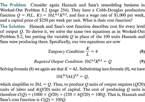
The Problem Consider again Hannah and Sam's remodeling business in Worked-Out Problem 8.2 (page 254). They have a Cobb-Douglas production function Q = F(L , K ) = 10 L 0.5 K 0.5 , and face a wage rate of $1,000 per week, and a capital price of $250 per week per unit. What is their cost function
The Solution Hannah and Sam's cost function describes cost for every level of output Q. To derive it, we solve the same two equations as in Worked-Out Problem 8.2, but putting the variable Q in place of the 100 units Hannah and Sam were producing there. Specifically, our two equations are now
Tangency Condition: = 4 (8)
Required Output Condition : 10 L 0.5 K 0.5 = Q (9)
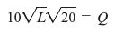
Solving formula (8) we again see that K = 4 L. Substituting into formula (9), we have
10 L 0.5 (4 L ) 0.5 = Q ,
which simplifies to 20 L = Q. Thus, to produce Q units of output requires ( Q /20) units of labor and 4( Q /20) units of capital. The cost of producing Q units is therefore C ( Q ) = (1000 × Q /20) + (250 × 4 Q /20) = 100 Q. That is, Hannah and Sam's cost function is C ( Q ) = 100 Q.
Worked-Out Problem 8.6
The Problem Consider again Hannah and Sam's remodeling business described in Worked-Out Problems 8.2 and 8.3 (pages 254 and 256). They have a Cobb-Douglas production function Q = F ( L , K ) = 10 L 0.5 K 0.5 , and face a wage rate of $1, 000 per week, and a capital price of $250 per week per unit. Suppose that they are initially remodeling 100 square feet per week using the least-cost input combination for producing that output level. What are their short-run and long-run cost functions if their capital is fixed in the short run, but variable in the long run
The Solution The solution to Worked-Out Problem 8.2 tells us that they initially use 20 units of capital. So, if their capital is fixed at 20 units, to remodel Q square feet Hannah and Sam need the amount of labor L that solves the formula
which means that L = ( Q 2 /2,000). So, their short-run cost function is
Or equivalently,
In contrast, the solution to Worked-Out Problem 8.3 tells us that Hannah and Sam's long-run cost function is
C LR ( Q ) = 100 Q
Observe, though, that their short-run and long-run costs are equal when Q = 100
, just as our discussion indicated they must be.Worked-Out Problem 8.2
Worked-Out Problem 8.3
The Problem Consider again Hannah and Sam's remodeling business in Worked-Out Problem 8.2 (page 254). They have a Cobb-Douglas production function Q = F(L , K ) = 10 L 0.5 K 0.5 , and face a wage rate of $1,000 per week, and a capital price of $250 per week per unit. What is their cost function
The Solution Hannah and Sam's cost function describes cost for every level of output Q. To derive it, we solve the same two equations as in Worked-Out Problem 8.2, but putting the variable Q in place of the 100 units Hannah and Sam were producing there. Specifically, our two equations are now
Tangency Condition: = 4 (8)
Required Output Condition : 10 L 0.5 K 0.5 = Q (9)
Solving formula (8) we again see that K = 4 L. Substituting into formula (9), we have
10 L 0.5 (4 L ) 0.5 = Q ,
which simplifies to 20 L = Q. Thus, to produce Q units of output requires ( Q /20) units of labor and 4( Q /20) units of capital. The cost of producing Q units is therefore C ( Q ) = (1000 × Q /20) + (250 × 4 Q /20) = 100 Q. That is, Hannah and Sam's cost function is C ( Q ) = 100 Q.
Question
Question

Unlock Deck
Sign up to unlock the cards in this deck!
Unlock Deck
Unlock Deck
1/37
Play
Full screen (f)
Deck 8: Cost
1
A firm has monthly production function
where L is worker hours per month and K is square feet of manufacturing space.
a. If the hourly wage rate is $50 and manufacturing space costs $25 per square foot per month, what is the firm's least-cost input combination for producing 100 units
b. Graph its output expansion path.
c. What is its cost function
where L is worker hours per month and K is square feet of manufacturing space.a. If the hourly wage rate is $50 and manufacturing space costs $25 per square foot per month, what is the firm's least-cost input combination for producing 100 units
b. Graph its output expansion path.
c. What is its cost function
The firm ABC's production function is given as:
 Where, L is worker hours per month and K is square feet of manufacturing space.
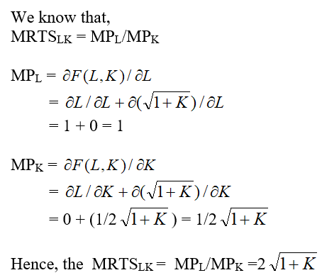
The Marginal Rate of Technical Substitution for firm ABC can be found out by the partial differentiation of it's production function.
 (a)The firm ABC's hourly wage rate W is $50 and manufacturing space costs R is $25 per square foot per month. To find the least cost combination of inputs to produce 100 units we need to determine the relation between the input quantities L and K.
We know that the marginal rate of technical substitution MRTS LK is same as the ratio of W and R.
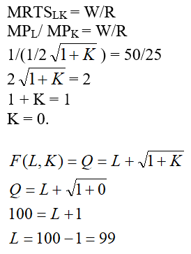 The above expression shows that the intersecting point between the two curves, that is the isoquant Q and isocost C, is at the axis where K = 0 and the value of L is 99.
(b)For the output expansion path, let us consider the values of Q as 10, 20, 30 and 40 for simplicity of the graph scope.
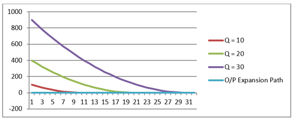 We can observe from the above graph that the least cost combination occurs when the isoquant touches the Labor axis K = 0. And hence, the output expansion path is also along the Labor axis.
(c)The Cost Function can be derived from the above found value of K = 0 (Tangency Condition).
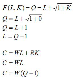 Hence, the cost function is

Where, L is worker hours per month and K is square feet of manufacturing space.The Marginal Rate of Technical Substitution for firm ABC can be found out by the partial differentiation of it's production function.
(a)The firm ABC's hourly wage rate W is $50 and manufacturing space costs R is $25 per square foot per month. To find the least cost combination of inputs to produce 100 units we need to determine the relation between the input quantities L and K.We know that the marginal rate of technical substitution MRTS LK is same as the ratio of W and R.
The above expression shows that the intersecting point between the two curves, that is the isoquant Q and isocost C, is at the axis where K = 0 and the value of L is 99. (b)For the output expansion path, let us consider the values of Q as 10, 20, 30 and 40 for simplicity of the graph scope.
We can observe from the above graph that the least cost combination occurs when the isoquant touches the Labor axis K = 0. And hence, the output expansion path is also along the Labor axis.(c)The Cost Function can be derived from the above found value of K = 0 (Tangency Condition).
Hence, the cost function is 2
Economist Milton Friedman is famous for remarking that "There is no such thing as a free lunch." Interpret this comment in light of the discussion in Section 8.2.
Introduction:
When a firm is decided to be set up, it incurs cost to be done so. Total cost is classified into two types viz. fixed cost plus variable cost.
For any firm to operate and earn profit in the market, it has to first incur some cost in order to start operating. This cost can be fixed cost or variable cost or combination of both. If fixed cost can be avoided it is known as avoidable cost but if the cost incurred can't be refunded, then such cost is sunk cost.
To summarize, nothing comes for free. To do business and earn revenue one has to first make some investment which includes cost. This explains the statement given in the question.
3
Suppose Noah and Naomi's short-run weekly production function is Q = F(L) = 2
and the wage rate is $12 an hour. Suppose also that the sunk cost (for their fixed garage-space input) is $500 per week. What is their short-run weekly cost function Graph this cost function.
and the wage rate is $12 an hour. Suppose also that the sunk cost (for their fixed garage-space input) is $500 per week. What is their short-run weekly cost function Graph this cost function.The objective of the following analysis is to derive the weekly cost function, given that the short-run production function is
 and the wage rate is $12 per hour and that the firm faces a sunk cost of $500 per week.
The short-run weekly production function is given by:
 This means,
 The sunk cost, which can be termed as total fixed cost is given by:
 The total variable cost is given by:
 Where,
 : Wage rate of $ 12 per hour
Thus, the weekly cost function is given by:
 Hence, the weekly cost function is:

and the wage rate is $12 per hour and that the firm faces a sunk cost of $500 per week.The short-run weekly production function is given by:
This means, The sunk cost, which can be termed as total fixed cost is given by: The total variable cost is given by: Where, : Wage rate of $ 12 per hourThus, the weekly cost function is given by:
Hence, the weekly cost function is: 4
Suppose Noah and Naomi's weekly production function for garden benches is F ( L ) = (3/2) L , where L represents the number of hours of labor employed. The wage rate is $15 an hour. What is their cost function
Unlock Deck
Unlock for access to all 37 flashcards in this deck.
Unlock Deck
k this deck
5
Suppose Alpha Corporation's daily cost function is C ( Q ) = Q 500 Q 2 + 2 Q 3. What is its efficient scale of production What is its minimum average cost
Unlock Deck
Unlock for access to all 37 flashcards in this deck.
Unlock Deck
k this deck
6
Many resort hotels remain open in the off season, even though they appear to be losing money. Why would they do so
Unlock Deck
Unlock for access to all 37 flashcards in this deck.
Unlock Deck
k this deck
7
Suppose a unit of capital instead costs Hannah and Sam $1,000 per week. Their production function and wage rate are the same as in Worked-Out Problem 8.2. What is their least-cost input combination for remodeling 100 square feet a week What is their total cost
Worked-Out Problem 8.2
Worked-Out Problem 8.2
Unlock Deck
Unlock for access to all 37 flashcards in this deck.
Unlock Deck
k this deck
8
Suppose Noah and Naomi's weekly production function for garden benches is F ( L ) = min{0, L 2}, where L represents the number of hours of labor employed. The wage rate is $15 an hour. What is their cost function
Unlock Deck
Unlock for access to all 37 flashcards in this deck.
Unlock Deck
k this deck
9
A firm has two production plants. The cost function of plant 1 is C 1 ( Q 1 ) = 10 Q 1 + ( Q 1 ) 2 where Q 1 is the number of units of output produced in plant 1. The cost function of plant 2 is C 2 ( Q 2 ) = 10 Q 2 + 4( Q 2 ) 2 where Q 2 is the number of units of output produced in plant 2. If the firm wants to produce Q total units of output, what is the allocation of production across the two plants that minimizes its cost
Unlock Deck
Unlock for access to all 37 flashcards in this deck.
Unlock Deck
k this deck
10
"A production method must be efficient to be a least-cost method of producing Q units of output, but an efficient method need not be a least-cost method." True or false Why
Unlock Deck
Unlock for access to all 37 flashcards in this deck.
Unlock Deck
k this deck
11
Suppose that a unit of capital instead costs Hannah and Sam $1,000 per week. (Their production function is the same as in worked- out problems 8.2 and 8.3.) What is their cost function
Unlock Deck
Unlock for access to all 37 flashcards in this deck.
Unlock Deck
k this deck
12
Johnson Tools produces hammers. It has signed a labor contract that guarantees its 1,000 workers a minimum of 30 hours per week of work. The contract also doubles the regular $20 per hour wage for overtime (more than 30 hours per week). Johnson's production technology uses only one variable input, labor. The company can produce two hammers per hour of employed labor. What is its variable cost function (assuming it cannot hire additional workers) Graph its variable cost curve.
Unlock Deck
Unlock for access to all 37 flashcards in this deck.
Unlock Deck
k this deck
13
Noah and Naomi want to produce 100 garden benches per week in two production plants. The cost functions at the two plants are C 1 ( Q 1 ) = 600 Q 1 3( Q 1 ) 2 and C 2 ( Q 2 ) = 650 Q 2 2( Q 2 ) 2. What is the best assignment of output between the two plants
Unlock Deck
Unlock for access to all 37 flashcards in this deck.
Unlock Deck
k this deck
14
Many airlines operate a hub-and-spoke system in which passengers headed for different destinations fly into the hub on the same plane, then switch planes to reach their final destinations. How does this system reflect the presence of economies of scope
Unlock Deck
Unlock for access to all 37 flashcards in this deck.
Unlock Deck
k this deck
15
Repeat worked-out problem 8.5, but assume instead that the total cost and marginal cost at plant 1 are C 1 = 6( Q 1 ) 2 and MC 1 = 12 Q 1 , respectively.
Unlock Deck
Unlock for access to all 37 flashcards in this deck.
Unlock Deck
k this deck
16
Suppose college graduates earn $25 an hour and high school graduates earn $15 an hour. Suppose too that the marginal product of college graduates at Johnson Tools is five hammers per hour, while the marginal product of high school graduates is four hammers per hour (regardless of the number of each type of worker employed). What is the least-cost production method for producing 100 hammers in an eight-hour day What if the marginal product of high school graduates were instead two hammers per hour What is the critical difference in productivity (in percentage terms) at which the type of worker hired changes
Unlock Deck
Unlock for access to all 37 flashcards in this deck.
Unlock Deck
k this deck
17
A firm that produces its output in Asia and sells it in the United States has one plant in country 1 and another in country 2. Both plants have production function F 1 ( L , K ) = LK. In country 1 the wage rate is W = 1 and the price of capital is R = 1. In country 2 the wage rate is W = 1 but the price of capital is R = 4. In addition, in country 1 any plant that operates must pay a permit fee of $20,000 per month, while in country 2 any plant that operates must pay a permit fee of $10,000 per month. The permit fee is an avoidable fixed cost: if the plant is shut down it doesn't need to be paid. Assume for simplicity in what follows that there are no costs of shipping the product from Asia to the United States.
a. What is the cost function, marginal cost function, and average cost function for each plant
b. What is the efficient scale and minimum average cost for each plant
c. What is the cost function for the firm
a. What is the cost function, marginal cost function, and average cost function for each plant
b. What is the efficient scale and minimum average cost for each plant
c. What is the cost function for the firm
Unlock Deck
Unlock for access to all 37 flashcards in this deck.
Unlock Deck
k this deck
18
What is Dan's efficient scale of production if his avoidable fixed cost is $605 per day What is his minimum average cost
Unlock Deck
Unlock for access to all 37 flashcards in this deck.
Unlock Deck
k this deck
19
Suppose that the production function for Hannah and Sam's home remodeling business is Q = F ( L , K ) = 10 L 0.2 K 0.3. If the wage rate is $1,500 per week and the cost of renting a unit of capital is $1,000 per week, what is the least-cost input combination for remodeling 100 square feet each week What is the total cost
Unlock Deck
Unlock for access to all 37 flashcards in this deck.
Unlock Deck
k this deck
20
The production function of a firm that uses labor ( L ) and capital ( K ) to produce its output is F ( L , K ) = 2 LK + K. The price of labor is $4 per unit and the price of capital is $5 per unit. If its level of capital is fixed in the short-run at K = 8, what is its cost of producing 40 units of output If it can vary its capital and labor freely in the long-run, what is its long-run cost of producing 40 units of output
Unlock Deck
Unlock for access to all 37 flashcards in this deck.
Unlock Deck
k this deck
21
Suppose that a unit of capital instead costs Hannah and Sam $1,000 per week. They are initially remodeling 100 square feet per week using the least-cost input combination for producing that output level. What are their short-run and long-run cost functions if their capital is fixed in the short run, but variable in the long run
Unlock Deck
Unlock for access to all 37 flashcards in this deck.
Unlock Deck
k this deck
22
Suppose that Hannah and Sam have the same production function as in Worked-Out Problem 8.2: Q = F ( L , K ) = 10 L 0.5 K 0.5. The wage rate is $1,000 per week and a unit of capital costs $250 per week. What is their least-cost input combination if they need to remodel 200 square feet per week What is their total cost
Worked-Out Problem 8.2
Worked-Out Problem 8.2
Unlock Deck
Unlock for access to all 37 flashcards in this deck.
Unlock Deck
k this deck
23
A firm's technology for producing its output from labor ( L ) and capital (K) is
. The wage is $2 per unit of labor and the cost of capital is $5 per unit of capital.
a. Does the firm's technology have a declining MRTS LK
b. What is the firm's cost function if both inputs are variable
c. Does the firm have economies of scale, diseconomies of scale, or neither
d. Suppose that the firm is initially producing 30 units of output. What is its cost function in the short run (when capital is fixed) Graph the long-run cost function and this short-run cost function in the same figure, labeling clearly all the important features such as where they each hit the vertical axis and any places they touch.
. The wage is $2 per unit of labor and the cost of capital is $5 per unit of capital.a. Does the firm's technology have a declining MRTS LK
b. What is the firm's cost function if both inputs are variable
c. Does the firm have economies of scale, diseconomies of scale, or neither
d. Suppose that the firm is initially producing 30 units of output. What is its cost function in the short run (when capital is fixed) Graph the long-run cost function and this short-run cost function in the same figure, labeling clearly all the important features such as where they each hit the vertical axis and any places they touch.
Unlock Deck
Unlock for access to all 37 flashcards in this deck.
Unlock Deck
k this deck
24
Suppose that Hannah and Sam's production function, wage rate, and price of capital are the same as in Problem 5. What is their cost function
Unlock Deck
Unlock for access to all 37 flashcards in this deck.
Unlock Deck
k this deck
25
Suppose that Hannah and Sam have the same production function as in Worked-Out Problem 8.2: Q = F ( L , K ) = 10 L 0.5 K 0.5. The wage rate is $1,000 per week and a unit of capital costs $4,000 per week. Graph their output expansion path. What is their cost function
Worked-Out Problem 8.2
Worked-Out Problem 8.2
Unlock Deck
Unlock for access to all 37 flashcards in this deck.
Unlock Deck
k this deck
26
(Calculus version below.) A firm has a monthly production function
, where L is hours of labor per month and K is square feet of manufacturing space. The marginal product of labor is MP L = 1, while the marginal product of capital is
.
a. If the hourly wage is $50 and manufacturing space costs $25 per square foot per month, what is the firm's least-cost input combination for producing 100 units
b. Graph its output expansion path.
c. What is its cost function
, where L is hours of labor per month and K is square feet of manufacturing space. The marginal product of labor is MP L = 1, while the marginal product of capital is .a. If the hourly wage is $50 and manufacturing space costs $25 per square foot per month, what is the firm's least-cost input combination for producing 100 units
b. Graph its output expansion path.
c. What is its cost function
Unlock Deck
Unlock for access to all 37 flashcards in this deck.
Unlock Deck
k this deck
27
Suppose that XYZ Corporation's total wages are twice the company's total expenditure on capital. XYZ has a Cobb-Douglas production function that has constant returns to scale. What can you deduce about parameters and of this production function
Unlock Deck
Unlock for access to all 37 flashcards in this deck.
Unlock Deck
k this deck
28
In December, Alpha Corp faced a wage rate of $10 per hour and a capital rental rate of $10 per unit per hour. It used 50 workers and 50 units of capital. In January, Alpha Corp faced a wage rate of $5 per hour and a capital rental rate of $10 per unit per hour. It used 10 workers and 60 units of capital. Which of the following input combinations must produce less output than the amount Alpha produced in December: ( L , K ) = (60, 60), ( L , K ) = (60, 40), ( L , K ) = (70, 30), and ( L , K ) = (80, 25)
Unlock Deck
Unlock for access to all 37 flashcards in this deck.
Unlock Deck
k this deck
29
Suppose that in worked-out problem 8.4 (page 271) Noah and Naomi wanted to produce 200 garden benches per week. What would be the best assignment of output to their two plants
Unlock Deck
Unlock for access to all 37 flashcards in this deck.
Unlock Deck
k this deck
30
(Suppose that Dan's Pizza Company in Worked-Out Problem 8.6 (page 271) instead has an avoidable fixed cost of $720 per day. What is his efficient scale of production What is his minimum average cost
Worked-Out Problem 8.6
The Problem Consider again Hannah and Sam's remodeling business described in Worked-Out Problems 8.2 and 8.3 (pages 254 and 256). They have a Cobb-Douglas production function Q = F ( L , K ) = 10 L 0.5 K 0.5 , and face a wage rate of $1, 000 per week, and a capital price of $250 per week per unit. Suppose that they are initially remodeling 100 square feet per week using the least-cost input combination for producing that output level. What are their short-run and long-run cost functions if their capital is fixed in the short run, but variable in the long run
The Solution The solution to Worked-Out Problem 8.2 tells us that they initially use 20 units of capital. So, if their capital is fixed at 20 units, to remodel Q square feet Hannah and Sam need the amount of labor L that solves the formula
which means that L = ( Q 2 /2,000). So, their short-run cost function is
Or equivalently,
In contrast, the solution to Worked-Out Problem 8.3 tells us that Hannah and Sam's long-run cost function is
C LR ( Q ) = 100 Q
Observe, though, that their short-run and long-run costs are equal when Q = 100
, just as our discussion indicated they must be.
Worked-Out Problem 8.2
Worked-Out Problem 8.3
Worked-Out Problem 8.6
The Problem Consider again Hannah and Sam's remodeling business described in Worked-Out Problems 8.2 and 8.3 (pages 254 and 256). They have a Cobb-Douglas production function Q = F ( L , K ) = 10 L 0.5 K 0.5 , and face a wage rate of $1, 000 per week, and a capital price of $250 per week per unit. Suppose that they are initially remodeling 100 square feet per week using the least-cost input combination for producing that output level. What are their short-run and long-run cost functions if their capital is fixed in the short run, but variable in the long run
The Solution The solution to Worked-Out Problem 8.2 tells us that they initially use 20 units of capital. So, if their capital is fixed at 20 units, to remodel Q square feet Hannah and Sam need the amount of labor L that solves the formula
which means that L = ( Q 2 /2,000). So, their short-run cost function is
Or equivalently,
In contrast, the solution to Worked-Out Problem 8.3 tells us that Hannah and Sam's long-run cost function is
C LR ( Q ) = 100 Q
Observe, though, that their short-run and long-run costs are equal when Q = 100
, just as our discussion indicated they must be.Worked-Out Problem 8.2
Worked-Out Problem 8.3
Unlock Deck
Unlock for access to all 37 flashcards in this deck.
Unlock Deck
k this deck
31
(Calculus version below.) Suppose Alpha Corporation's daily cost function is C ( Q ) = Q 500 Q + 2 Q 3. It's marginal cost is C ( Q ) = 1 1000 Q 2 + 6 Q 2. What is its efficient scale of production What is its minimum average cost
Unlock Deck
Unlock for access to all 37 flashcards in this deck.
Unlock Deck
k this deck
32
(Suppose that in Worked-Out Problem 8.4 (page 261), the cost function at plant 2 was C 2 ( Q 2 ) = 650 Q 2 + 2( Q 2 ) 2 , and marginal cost at that plant was MC 2 = 650 + 4 Q 2. What would be the best assignment of output between the two plants
Worked-Out Problem 8.4
The Problem Suppose Noah and Naomi have just acquired a second garden bench production plant. Production costs are C 1 ( Q 1 ) = 3( Q 1 ) 2 at plant 1 and C 2 (Q 2 ) = 2( Q 2 ) 2 at plant 2, where Q 1 and Q 2 are the number of benches produced at each plant per week. The corresponding marginal costs at the two plants are MC 1 = 6 Q 1 and MC 2 = 4 Q 2. If Noah and Naomi plan to produce 100 benches per week and want to do it as economically as possible, how many benches should they produce at each plant
The Solution The basic principle behind the solution to this problem is similar to that in Worked-Out Problem 7.1 (page 216). With a least-cost plan that assigns a positive amount of output to each plant, marginal cost must be the same at both plants. If that were not true, the total cost could be lowered by reassigning a little bit of output from the plant with the higher marginal cost to the plant with the lower marginal cost.
Noah and Naomi need to divide production between the two plants so that their marginal costs are equal. Doing so means choosing Q 1 and Q 2 so that MC 1 = MC 2. Since total output equals 100, we know that Q 2 = 100 Q 1 , so we can express the marginal cost in plant 2 as a function of the amount of output produced in plant 1: MC 2 = 4(100 - Q 1 ). We can then find the output assignment that equates marginal costs in the two plants by solving the formula
6 Q 1 = 4(100 - Q 1 )The solution is Q 1 = 40. Noah and Naomi should produce 40 garden benches a week in plant 1 and 60 garden benches a week in plant 2. Their total production costs will then be
C = 3(40) 2 + 2(60) 2 = $12,000
Worked-Out Problem 7.1
The Problem John, April, and Tristan own JATjuice, a firm that produces freshly squeezed orange juice. Oranges are their only variable input. They have two production facilities. Suppose the marginal product of oranges in plant 1 is
, where O 1 is the number of crates of oranges allocated to plant 1. The marginal product of oranges in plant 2 is
, where O 2 is the number of crates of oranges assigned to plant 2. Suppose that John, April, and Tristan have a total of 600 crates of oranges. What is the best assignment of oranges to the two plants
The Solution Start by writing the marginal product in plant 2asa function of the number of crates of oranges assigned to plant 1, O 1 :
Now find the level of O 1 that equates the marginal product of oranges in the two plants. We can do so with algebra by setting
and solving:
John, April, and Tristan should assign 200 crates to plant 1 and the rest (400) to plant 2.
Worked-Out Problem 8.4
The Problem Suppose Noah and Naomi have just acquired a second garden bench production plant. Production costs are C 1 ( Q 1 ) = 3( Q 1 ) 2 at plant 1 and C 2 (Q 2 ) = 2( Q 2 ) 2 at plant 2, where Q 1 and Q 2 are the number of benches produced at each plant per week. The corresponding marginal costs at the two plants are MC 1 = 6 Q 1 and MC 2 = 4 Q 2. If Noah and Naomi plan to produce 100 benches per week and want to do it as economically as possible, how many benches should they produce at each plant
The Solution The basic principle behind the solution to this problem is similar to that in Worked-Out Problem 7.1 (page 216). With a least-cost plan that assigns a positive amount of output to each plant, marginal cost must be the same at both plants. If that were not true, the total cost could be lowered by reassigning a little bit of output from the plant with the higher marginal cost to the plant with the lower marginal cost.
Noah and Naomi need to divide production between the two plants so that their marginal costs are equal. Doing so means choosing Q 1 and Q 2 so that MC 1 = MC 2. Since total output equals 100, we know that Q 2 = 100 Q 1 , so we can express the marginal cost in plant 2 as a function of the amount of output produced in plant 1: MC 2 = 4(100 - Q 1 ). We can then find the output assignment that equates marginal costs in the two plants by solving the formula
6 Q 1 = 4(100 - Q 1 )The solution is Q 1 = 40. Noah and Naomi should produce 40 garden benches a week in plant 1 and 60 garden benches a week in plant 2. Their total production costs will then be
C = 3(40) 2 + 2(60) 2 = $12,000
Worked-Out Problem 7.1
The Problem John, April, and Tristan own JATjuice, a firm that produces freshly squeezed orange juice. Oranges are their only variable input. They have two production facilities. Suppose the marginal product of oranges in plant 1 is
, where O 1 is the number of crates of oranges allocated to plant 1. The marginal product of oranges in plant 2 is , where O 2 is the number of crates of oranges assigned to plant 2. Suppose that John, April, and Tristan have a total of 600 crates of oranges. What is the best assignment of oranges to the two plants The Solution Start by writing the marginal product in plant 2asa function of the number of crates of oranges assigned to plant 1, O 1 :
Now find the level of O 1 that equates the marginal product of oranges in the two plants. We can do so with algebra by setting
and solving: John, April, and Tristan should assign 200 crates to plant 1 and the rest (400) to plant 2.
Unlock Deck
Unlock for access to all 37 flashcards in this deck.
Unlock Deck
k this deck
33
(Calculus version below.) Noah and Naomi want to produce 100 garden benches per week in two production plants. The cost functions at the two plants are C 1 ( Q 1 ) = 600 Q 1 3( Q 1 ) 2 and C 2 ( Q 2 ) = 650 Q 2 2( Q 2 ) and the corresponding marginal costs are MC 1 = 600 6 Q 1 and MC 2 = 650 4 Q 2. What is the best assignment of output between the two plants
Unlock Deck
Unlock for access to all 37 flashcards in this deck.
Unlock Deck
k this deck
34
(Consider again Worked-Out Problem 8.6 (page 271) but assume that Hannah and Sam are initially remodeling 200 square feet per week. What are their short-run and long-run cost functions if capital is fixed in the short run, but variable in the long run
Worked-Out Problem 8.6
The Problem Consider again Hannah and Sam's remodeling business described in Worked-Out Problems 8.2 and 8.3 (pages 254 and 256). They have a Cobb-Douglas production function Q = F ( L , K ) = 10 L 0.5 K 0.5 , and face a wage rate of $1, 000 per week, and a capital price of $250 per week per unit. Suppose that they are initially remodeling 100 square feet per week using the least-cost input combination for producing that output level. What are their short-run and long-run cost functions if their capital is fixed in the short run, but variable in the long run
The Solution The solution to Worked-Out Problem 8.2 tells us that they initially use 20 units of capital. So, if their capital is fixed at 20 units, to remodel Q square feet Hannah and Sam need the amount of labor L that solves the formula
which means that L = ( Q 2 /2,000). So, their short-run cost function is
Or equivalently,
In contrast, the solution to Worked-Out Problem 8.3 tells us that Hannah and Sam's long-run cost function is
C LR ( Q ) = 100 Q
Observe, though, that their short-run and long-run costs are equal when Q = 100
, just as our discussion indicated they must be.
Worked-Out Problem 8.2
Worked-Out Problem 8.3
Worked-Out Problem 8.6
The Problem Consider again Hannah and Sam's remodeling business described in Worked-Out Problems 8.2 and 8.3 (pages 254 and 256). They have a Cobb-Douglas production function Q = F ( L , K ) = 10 L 0.5 K 0.5 , and face a wage rate of $1, 000 per week, and a capital price of $250 per week per unit. Suppose that they are initially remodeling 100 square feet per week using the least-cost input combination for producing that output level. What are their short-run and long-run cost functions if their capital is fixed in the short run, but variable in the long run
The Solution The solution to Worked-Out Problem 8.2 tells us that they initially use 20 units of capital. So, if their capital is fixed at 20 units, to remodel Q square feet Hannah and Sam need the amount of labor L that solves the formula
which means that L = ( Q 2 /2,000). So, their short-run cost function is
Or equivalently,
In contrast, the solution to Worked-Out Problem 8.3 tells us that Hannah and Sam's long-run cost function is
C LR ( Q ) = 100 Q
Observe, though, that their short-run and long-run costs are equal when Q = 100
, just as our discussion indicated they must be.Worked-Out Problem 8.2
Worked-Out Problem 8.3
Unlock Deck
Unlock for access to all 37 flashcards in this deck.
Unlock Deck
k this deck
35
Consider again Worked-Out Problem 8.6 (page 271) but assume that a unit of capital costs $1,000 per week and that Hannah and Sam are initially remodeling 200 square feet per week. What are their short-run and long-run cost functions if capital is fixed in the short run, but variable in the long run
Worked-Out Problem 8.6
The Problem Consider again Hannah and Sam's remodeling business described in Worked-Out Problems 8.2 and 8.3 (pages 254 and 256). They have a Cobb-Douglas production function Q = F ( L , K ) = 10 L 0.5 K 0.5 , and face a wage rate of $1, 000 per week, and a capital price of $250 per week per unit. Suppose that they are initially remodeling 100 square feet per week using the least-cost input combination for producing that output level. What are their short-run and long-run cost functions if their capital is fixed in the short run, but variable in the long run
The Solution The solution to Worked-Out Problem 8.2 tells us that they initially use 20 units of capital. So, if their capital is fixed at 20 units, to remodel Q square feet Hannah and Sam need the amount of labor L that solves the formula
which means that L = ( Q 2 /2,000). So, their short-run cost function is
Or equivalently,
In contrast, the solution to Worked-Out Problem 8.3 tells us that Hannah and Sam's long-run cost function is
C LR ( Q ) = 100 Q
Observe, though, that their short-run and long-run costs are equal when Q = 100
, just as our discussion indicated they must be.
Worked-Out Problem 8.2
Worked-Out Problem 8.3
The Problem Consider again Hannah and Sam's remodeling business in Worked-Out Problem 8.2 (page 254). They have a Cobb-Douglas production function Q = F(L , K ) = 10 L 0.5 K 0.5 , and face a wage rate of $1,000 per week, and a capital price of $250 per week per unit. What is their cost function
The Solution Hannah and Sam's cost function describes cost for every level of output Q. To derive it, we solve the same two equations as in Worked-Out Problem 8.2, but putting the variable Q in place of the 100 units Hannah and Sam were producing there. Specifically, our two equations are now
Tangency Condition: = 4 (8)
Required Output Condition : 10 L 0.5 K 0.5 = Q (9)
Solving formula (8) we again see that K = 4 L. Substituting into formula (9), we have
10 L 0.5 (4 L ) 0.5 = Q ,
which simplifies to 20 L = Q. Thus, to produce Q units of output requires ( Q /20) units of labor and 4( Q /20) units of capital. The cost of producing Q units is therefore C ( Q ) = (1000 × Q /20) + (250 × 4 Q /20) = 100 Q. That is, Hannah and Sam's cost function is C ( Q ) = 100 Q.
Worked-Out Problem 8.6
The Problem Consider again Hannah and Sam's remodeling business described in Worked-Out Problems 8.2 and 8.3 (pages 254 and 256). They have a Cobb-Douglas production function Q = F ( L , K ) = 10 L 0.5 K 0.5 , and face a wage rate of $1, 000 per week, and a capital price of $250 per week per unit. Suppose that they are initially remodeling 100 square feet per week using the least-cost input combination for producing that output level. What are their short-run and long-run cost functions if their capital is fixed in the short run, but variable in the long run
The Solution The solution to Worked-Out Problem 8.2 tells us that they initially use 20 units of capital. So, if their capital is fixed at 20 units, to remodel Q square feet Hannah and Sam need the amount of labor L that solves the formula
which means that L = ( Q 2 /2,000). So, their short-run cost function is
Or equivalently,
In contrast, the solution to Worked-Out Problem 8.3 tells us that Hannah and Sam's long-run cost function is
C LR ( Q ) = 100 Q
Observe, though, that their short-run and long-run costs are equal when Q = 100
, just as our discussion indicated they must be.Worked-Out Problem 8.2
Worked-Out Problem 8.3
The Problem Consider again Hannah and Sam's remodeling business in Worked-Out Problem 8.2 (page 254). They have a Cobb-Douglas production function Q = F(L , K ) = 10 L 0.5 K 0.5 , and face a wage rate of $1,000 per week, and a capital price of $250 per week per unit. What is their cost function
The Solution Hannah and Sam's cost function describes cost for every level of output Q. To derive it, we solve the same two equations as in Worked-Out Problem 8.2, but putting the variable Q in place of the 100 units Hannah and Sam were producing there. Specifically, our two equations are now
Tangency Condition: = 4 (8)
Required Output Condition : 10 L 0.5 K 0.5 = Q (9)
Solving formula (8) we again see that K = 4 L. Substituting into formula (9), we have
10 L 0.5 (4 L ) 0.5 = Q ,
which simplifies to 20 L = Q. Thus, to produce Q units of output requires ( Q /20) units of labor and 4( Q /20) units of capital. The cost of producing Q units is therefore C ( Q ) = (1000 × Q /20) + (250 × 4 Q /20) = 100 Q. That is, Hannah and Sam's cost function is C ( Q ) = 100 Q.
Unlock Deck
Unlock for access to all 37 flashcards in this deck.
Unlock Deck
k this deck
36
Suppose that Hannah and Sam have the Cobb- Douglas production function Q = F ( L, K ) = 10 L 0.25 K 0 25. Both a worker and a unit of capital cost $1,000 per week. If Hannah and Sam begin by remodeling 100 square feet per week, and if their capital is fixed in the short run but variable in the long run, what are their long-run and short-run cost functions What are their long-run and short-run average cost functions for positive output levels
Unlock Deck
Unlock for access to all 37 flashcards in this deck.
Unlock Deck
k this deck
37
Does a firm with the cost function C ( Q ) = Q 2 experience economies of scale, diseconomies of scale, or neither
Unlock Deck
Unlock for access to all 37 flashcards in this deck.
Unlock Deck
k this deck
Unlock Deck
Unlock for access to all 37 flashcards in this deck.


