Deck 2: Exploring Data Patterns and Choosing a Forecasting Technique
Full screen (f)
Question
Question
Question
Question
Question
Question
Question
Question
Question
Question
Question
Question
Question
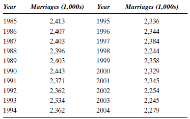
The number of marriages in the United States is given in Table P-13. Compute the first differences for these data. Plot the original data and the difference data as a time series. Is there a trend in either of these series? Discuss.
TABLE P-13
Source: Based on Statistical Abstract of the United States, various years.
TABLE P-13
Source: Based on Statistical Abstract of the United States, various years.
Question
Question
Question
Question
Allie White, the chief loan officer for the Dominion Bank, would like to analyze the bank's loan portfolio for the years 2001 to 2006. The data are shown in Table P-17.
a. Compute the autocorrelations for time lags 1 and 2. Test to determine whether these autocorrelation coefficients are significantly different from zero at the.05 significance level.
b. Use a computer program to plot the data and compute the autocorrelations for the first six time lags. Is this time series stationary?
TABLE P-17 Quarterly Loans ($ millions) for Dominion Bank, 2001-2006
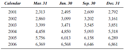
Source: Based on Dominion Bank records.
a. Compute the autocorrelations for time lags 1 and 2. Test to determine whether these autocorrelation coefficients are significantly different from zero at the.05 significance level.
b. Use a computer program to plot the data and compute the autocorrelations for the first six time lags. Is this time series stationary?
TABLE P-17 Quarterly Loans ($ millions) for Dominion Bank, 2001-2006
Source: Based on Dominion Bank records.
Question
Question
Analyze the autocorrelation coefficients for the series shown in Figures 3-18 through 3-21. Briefly describe each series.
FIGURE 3-18 Autocorrelation Function
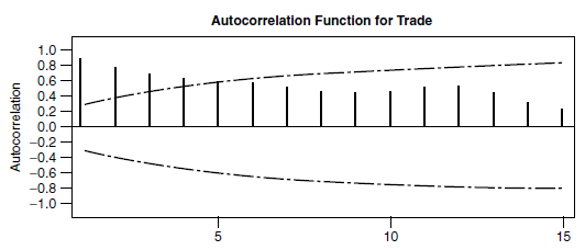
FIGURE 3-19 Autocorrelation Function
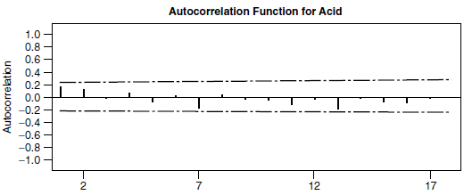
FIGURE 3-20 Autocorrelation Function
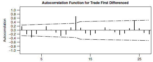
FIGURE 3-21 Autocorrelation Function
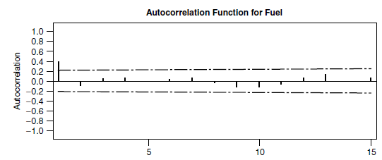
FIGURE 3-18 Autocorrelation Function
FIGURE 3-19 Autocorrelation Function
FIGURE 3-20 Autocorrelation Function
FIGURE 3-21 Autocorrelation Function
Question
An analyst would like to determine whether there is a pattern to earnings per share for the Price Company, which operated a wholesale/retail cash-and-carry business in several states under the name Price Club. The data are shown in Table P-20. Describe any patterns that exist in these data.
a. Find the forecast value of the quarterly earnings per share for Price Club for each quarter by using the naive approach (i.e., the forecast for first-quarter 1987 is the value for fourth-quarter 1986,.32).
b. Evaluate the naive forecast using MAD.
c. Evaluate the naive forecast using MSE and RMSE.
d. Evaluate the naive forecast using MAPE.
e. Evaluate the naive forecast using MPE.
TABLE P-20 Quarterly Earnings per Share for Price Club: 1986-1993 Quarter
Source: The Value Line Investment Survey (New York: Value Line, 1994), p. 1646.
Question
Table P-21 contains the weekly sales for a food item for 52 consecutive weeks.
a. Plot the sales data as a time series.
b. Do you think this series is stationary or nonstationary?
c. Using Minitab or a similar program, compute the autocorrelations of the sales series for the first 10 time lags. Is the behavior of the autocorrelations consistent with your choice in part b? Explain.
TABLE P-21 Weekly Sales of a Food Item
Question
This question refers to Problem 21.
a. Fit the random model given by Equation 3.4 to the data in Table P-21 by estimating c with the sample mean
 so
so
 . Compute the residuals using
 .
.
b. Using Minitab or a similar program, compute the autocorrelations of the residuals from part c for the first 10 time lags. Is the random model adequate for the sales data? Explain.
TABLE P-21 Weekly Sales of a Food Item

a. Fit the random model given by Equation 3.4 to the data in Table P-21 by estimating c with the sample mean
so . Compute the residuals using .b. Using Minitab or a similar program, compute the autocorrelations of the residuals from part c for the first 10 time lags. Is the random model adequate for the sales data? Explain.
TABLE P-21 Weekly Sales of a Food Item
Question
Table P-23 contains Southwest Airlines' quarterly income before extraordinary items ($MM) for the years 1988-1999.
a. Plot the income data as a time series and describe any patterns that exist.
b. Is this series stationary or nonstationary? Explain.
c. Using Minitab or a similar program, compute the autocorrelations of the income series for the first 10 time lags. Is the behavior of the autocorrelations consistent with your choice in part b? Explain.
TABLE P-23 Quarterly Income for Southwest Airlines ($MM)
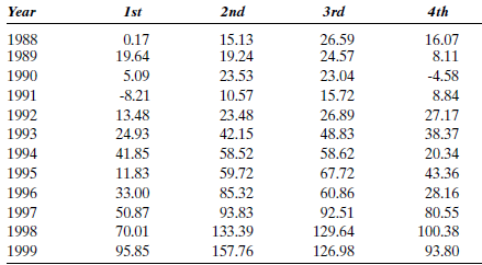
Source: Based on Compustat Industrial Quarterly Data Base
a. Plot the income data as a time series and describe any patterns that exist.
b. Is this series stationary or nonstationary? Explain.
c. Using Minitab or a similar program, compute the autocorrelations of the income series for the first 10 time lags. Is the behavior of the autocorrelations consistent with your choice in part b? Explain.
TABLE P-23 Quarterly Income for Southwest Airlines ($MM)
Source: Based on Compustat Industrial Quarterly Data Base
Question
This question refers to Problem 23.
a. Use Minitab or Excel to compute the fourth differences of the income data in Table P-23. Fourth differences are computed by differencing observations four time periods apart. With quarterly data, this procedure is sometimes useful for creating a stationary series from a nonstationary series (see Chapter 9). Consequently, the fourth differenced data will be Y 5 ? Y 1 = 19.64 ?.17 = 19.47, Y 6 ? Y 2 = 19.24 ? 15.13 = 4.11,... , and so forth.
b. Plot the time series of fourth differences. Does this time series appear to be stationary or nonstationary? Explain.
TABLE P-23 Quarterly Income for Southwest Airlines ($MM)

Source: Based on Compustat Industrial Quarterly Data Base
a. Use Minitab or Excel to compute the fourth differences of the income data in Table P-23. Fourth differences are computed by differencing observations four time periods apart. With quarterly data, this procedure is sometimes useful for creating a stationary series from a nonstationary series (see Chapter 9). Consequently, the fourth differenced data will be Y 5 ? Y 1 = 19.64 ?.17 = 19.47, Y 6 ? Y 2 = 19.24 ? 15.13 = 4.11,... , and so forth.
b. Plot the time series of fourth differences. Does this time series appear to be stationary or nonstationary? Explain.
TABLE P-23 Quarterly Income for Southwest Airlines ($MM)
Source: Based on Compustat Industrial Quarterly Data Base
Question
This question refers to Problem 23.
TABLE P-23 Quarterly Income for Southwest Airlines ($MM)

Source: Based on Compustat Industrial Quarterly Data Base.
a. Consider a naive forecasting method where the first-quarter income is used to forecast first-quarter income for the following year, second-quarter income is used to forecast second-quarter income, and so forth. For example, a forecast of first-quarter income for 1998 is provided by the first-quarter income for 1997, 50.87 (see Table P-23). Use this naive method to calculate forecasts of quarterly income for the years 1998-1999.
b. Using the forecasts in part a, calculate the MAD, RMSE, and MAPE.
c. Given the results in part b and the nature of the patterns in the income series, do you think this naive forecasting method is viable? Can you think of another naive method that might be better?
TABLE P-23 Quarterly Income for Southwest Airlines ($MM)
Source: Based on Compustat Industrial Quarterly Data Base.
a. Consider a naive forecasting method where the first-quarter income is used to forecast first-quarter income for the following year, second-quarter income is used to forecast second-quarter income, and so forth. For example, a forecast of first-quarter income for 1998 is provided by the first-quarter income for 1997, 50.87 (see Table P-23). Use this naive method to calculate forecasts of quarterly income for the years 1998-1999.
b. Using the forecasts in part a, calculate the MAD, RMSE, and MAPE.
c. Given the results in part b and the nature of the patterns in the income series, do you think this naive forecasting method is viable? Can you think of another naive method that might be better?
Question
MURPHY BROTHERS FURNITURE
In 1958, the Murphy brothers established a furniture store in downtown Dallas. Over the years, they were quite successful and extended their retail coverage throughout the West and Midwest. By 1996, their chain of furniture stores had become well established in 36 states.
Julie Murphy, the daughter of one of the founders, had recently joined the firm. Her father and uncle were sophisticated in many ways but not in the area of quantitative skills. In particular, they both felt that they could not accurately forecast the future sales of Murphy Brothers using modern computer techniques. For this reason, they appealed to Julie for help as part of her new job.
Julie first considered using Murphy sales dollars as her variable but found that several years of history were missing. She asked her father, Glen, about this, and he told her that at the time he "didn't think it was that important." Julie explained the importance of past data to Glen, and he indicated that he would save future data.
Julie decided that Murphy sales were probably closely related to national sales figures and decided to search for an appropriate variable in one of the many federal publications. After looking through a recent copy of the Survey of Current Business, she found the history on monthly sales for all retail stores in the United States and decided to use this variable as a substitute for her variable of interest, Murphy Brothers sales dollars. She reasoned that, if she could establish accurate forecasts for national sales, she could relate these forecasts to Murphy's own sales and come up with the forecasts she wanted.
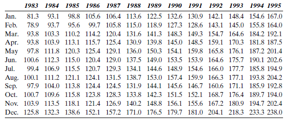
Table 3-8 shows the data that Julie collected, and Figure 3-22 shows a data plot provided by Julie's computer program. Julie began her analysis by using the computer to develop a plot of the autocorrelation coefficients.
After examining the autocorrelation function produced in Figure 3-23, it was obvious to Julie that her data contain a trend. The early autocorrelation coefficients are very large, and they drop toward zero very slowly with time. To make the series stationary so that various forecasting methods could be considered, Julie decided to first difference her data to see if the trend could be removed. The autocorrelation function for the first differenced data is shown in Figure 3-24.
TABLE 3-8 Monthly Sales ($ billions) for All Retail Stores, 1983-1995

Source: Based on Survey of Current Business , various years.
FIGURE 3-22 Time Series Graph of Monthly Sales for All U.S. Retail Stores, 1983-1995
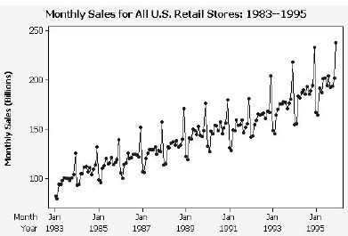
FIGURE 3-23 Autocorrelation Function for Monthly Sales for All U.S. Retail Stores
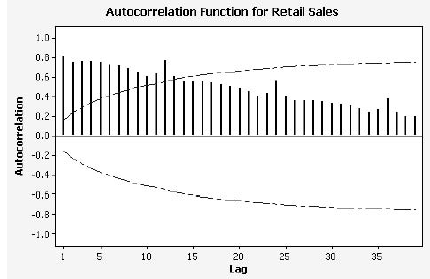
FIGURE 3-24 Autocorrelation Function for Monthly Sales for All U.S. Retail Stores First Differenced

What should Julie conclude about the retail sales series?
In 1958, the Murphy brothers established a furniture store in downtown Dallas. Over the years, they were quite successful and extended their retail coverage throughout the West and Midwest. By 1996, their chain of furniture stores had become well established in 36 states.
Julie Murphy, the daughter of one of the founders, had recently joined the firm. Her father and uncle were sophisticated in many ways but not in the area of quantitative skills. In particular, they both felt that they could not accurately forecast the future sales of Murphy Brothers using modern computer techniques. For this reason, they appealed to Julie for help as part of her new job.
Julie first considered using Murphy sales dollars as her variable but found that several years of history were missing. She asked her father, Glen, about this, and he told her that at the time he "didn't think it was that important." Julie explained the importance of past data to Glen, and he indicated that he would save future data.
Julie decided that Murphy sales were probably closely related to national sales figures and decided to search for an appropriate variable in one of the many federal publications. After looking through a recent copy of the Survey of Current Business, she found the history on monthly sales for all retail stores in the United States and decided to use this variable as a substitute for her variable of interest, Murphy Brothers sales dollars. She reasoned that, if she could establish accurate forecasts for national sales, she could relate these forecasts to Murphy's own sales and come up with the forecasts she wanted.
Table 3-8 shows the data that Julie collected, and Figure 3-22 shows a data plot provided by Julie's computer program. Julie began her analysis by using the computer to develop a plot of the autocorrelation coefficients.
After examining the autocorrelation function produced in Figure 3-23, it was obvious to Julie that her data contain a trend. The early autocorrelation coefficients are very large, and they drop toward zero very slowly with time. To make the series stationary so that various forecasting methods could be considered, Julie decided to first difference her data to see if the trend could be removed. The autocorrelation function for the first differenced data is shown in Figure 3-24.
TABLE 3-8 Monthly Sales ($ billions) for All Retail Stores, 1983-1995
Source: Based on Survey of Current Business , various years.
FIGURE 3-22 Time Series Graph of Monthly Sales for All U.S. Retail Stores, 1983-1995
FIGURE 3-23 Autocorrelation Function for Monthly Sales for All U.S. Retail Stores
FIGURE 3-24 Autocorrelation Function for Monthly Sales for All U.S. Retail Stores First Differenced
What should Julie conclude about the retail sales series?
Question
MURPHY BROTHERS FURNITURE
In 1958, the Murphy brothers established a furniture store in downtown Dallas. Over the years, they were quite successful and extended their retail coverage throughout the West and Midwest. By 1996, their chain of furniture stores had become well established in 36 states.
Julie Murphy, the daughter of one of the founders, had recently joined the firm. Her father and uncle were sophisticated in many ways but not in the area of quantitative skills. In particular, they both felt that they could not accurately forecast the future sales of Murphy Brothers using modern computer techniques. For this reason, they appealed to Julie for help as part of her new job.
Julie first considered using Murphy sales dollars as her variable but found that several years of history were missing. She asked her father, Glen, about this, and he told her that at the time he "didn't think it was that important." Julie explained the importance of past data to Glen, and he indicated that he would save future data.
Julie decided that Murphy sales were probably closely related to national sales figures and decided to search for an appropriate variable in one of the many federal publications. After looking through a recent copy of the Survey of Current Business, she found the history on monthly sales for all retail stores in the United States and decided to use this variable as a substitute for her variable of interest, Murphy Brothers sales dollars. She reasoned that, if she could establish accurate forecasts for national sales, she could relate these forecasts to Murphy's own sales and come up with the forecasts she wanted.
Table 3-8 shows the data that Julie collected, and Figure 3-22 shows a data plot provided by Julie's computer program. Julie began her analysis by using the computer to develop a plot of the autocorrelation coefficients.
After examining the autocorrelation function produced in Figure 3-23, it was obvious to Julie that her data contain a trend. The early autocorrelation coefficients are very large, and they drop toward zero very slowly with time. To make the series stationary so that various forecasting methods could be considered, Julie decided to first difference her data to see if the trend could be removed. The autocorrelation function for the first differenced data is shown in Figure 3-24.
TABLE 3-8 Monthly Sales ($ billions) for All Retail Stores, 1983-1995

Source: Based on Survey of Current Business , various years.
FIGURE 3-22 Time Series Graph of Monthly Sales for All U.S. Retail Stores, 1983-1995

FIGURE 3-23 Autocorrelation Function for Monthly Sales for All U.S. Retail Stores

FIGURE 3-24 Autocorrelation Function for Monthly Sales for All U.S. Retail Stores First Differenced

Has Julie made good progress toward finding a forecasting technique?
In 1958, the Murphy brothers established a furniture store in downtown Dallas. Over the years, they were quite successful and extended their retail coverage throughout the West and Midwest. By 1996, their chain of furniture stores had become well established in 36 states.
Julie Murphy, the daughter of one of the founders, had recently joined the firm. Her father and uncle were sophisticated in many ways but not in the area of quantitative skills. In particular, they both felt that they could not accurately forecast the future sales of Murphy Brothers using modern computer techniques. For this reason, they appealed to Julie for help as part of her new job.
Julie first considered using Murphy sales dollars as her variable but found that several years of history were missing. She asked her father, Glen, about this, and he told her that at the time he "didn't think it was that important." Julie explained the importance of past data to Glen, and he indicated that he would save future data.
Julie decided that Murphy sales were probably closely related to national sales figures and decided to search for an appropriate variable in one of the many federal publications. After looking through a recent copy of the Survey of Current Business, she found the history on monthly sales for all retail stores in the United States and decided to use this variable as a substitute for her variable of interest, Murphy Brothers sales dollars. She reasoned that, if she could establish accurate forecasts for national sales, she could relate these forecasts to Murphy's own sales and come up with the forecasts she wanted.
Table 3-8 shows the data that Julie collected, and Figure 3-22 shows a data plot provided by Julie's computer program. Julie began her analysis by using the computer to develop a plot of the autocorrelation coefficients.
After examining the autocorrelation function produced in Figure 3-23, it was obvious to Julie that her data contain a trend. The early autocorrelation coefficients are very large, and they drop toward zero very slowly with time. To make the series stationary so that various forecasting methods could be considered, Julie decided to first difference her data to see if the trend could be removed. The autocorrelation function for the first differenced data is shown in Figure 3-24.
TABLE 3-8 Monthly Sales ($ billions) for All Retail Stores, 1983-1995
Source: Based on Survey of Current Business , various years.
FIGURE 3-22 Time Series Graph of Monthly Sales for All U.S. Retail Stores, 1983-1995
FIGURE 3-23 Autocorrelation Function for Monthly Sales for All U.S. Retail Stores
FIGURE 3-24 Autocorrelation Function for Monthly Sales for All U.S. Retail Stores First Differenced
Has Julie made good progress toward finding a forecasting technique?
Question
MURPHY BROTHERS FURNITURE
In 1958, the Murphy brothers established a furniture store in downtown Dallas. Over the years, they were quite successful and extended their retail coverage throughout the West and Midwest. By 1996, their chain of furniture stores had become well established in 36 states.
Julie Murphy, the daughter of one of the founders, had recently joined the firm. Her father and uncle were sophisticated in many ways but not in the area of quantitative skills. In particular, they both felt that they could not accurately forecast the future sales of Murphy Brothers using modern computer techniques. For this reason, they appealed to Julie for help as part of her new job.
Julie first considered using Murphy sales dollars as her variable but found that several years of history were missing. She asked her father, Glen, about this, and he told her that at the time he "didn't think it was that important." Julie explained the importance of past data to Glen, and he indicated that he would save future data.
Julie decided that Murphy sales were probably closely related to national sales figures and decided to search for an appropriate variable in one of the many federal publications. After looking through a recent copy of the Survey of Current Business, she found the history on monthly sales for all retail stores in the United States and decided to use this variable as a substitute for her variable of interest, Murphy Brothers sales dollars. She reasoned that, if she could establish accurate forecasts for national sales, she could relate these forecasts to Murphy's own sales and come up with the forecasts she wanted.
Table 3-8 shows the data that Julie collected, and Figure 3-22 shows a data plot provided by Julie's computer program. Julie began her analysis by using the computer to develop a plot of the autocorrelation coefficients.
After examining the autocorrelation function produced in Figure 3-23, it was obvious to Julie that her data contain a trend. The early autocorrelation coefficients are very large, and they drop toward zero very slowly with time. To make the series stationary so that various forecasting methods could be considered, Julie decided to first difference her data to see if the trend could be removed. The autocorrelation function for the first differenced data is shown in Figure 3-24.
TABLE 3-8 Monthly Sales ($ billions) for All Retail Stores, 1983-1995
Source: Based on Survey of Current Business , various years.
FIGURE 3-22 Time Series Graph of Monthly Sales for All U.S. Retail Stores, 1983-1995

FIGURE 3-23 Autocorrelation Function for Monthly Sales for All U.S. Retail Stores

FIGURE 3-24 Autocorrelation Function for Monthly Sales for All U.S. Retail Stores First Differenced
What forecasting techniques should Julie try?
In 1958, the Murphy brothers established a furniture store in downtown Dallas. Over the years, they were quite successful and extended their retail coverage throughout the West and Midwest. By 1996, their chain of furniture stores had become well established in 36 states.
Julie Murphy, the daughter of one of the founders, had recently joined the firm. Her father and uncle were sophisticated in many ways but not in the area of quantitative skills. In particular, they both felt that they could not accurately forecast the future sales of Murphy Brothers using modern computer techniques. For this reason, they appealed to Julie for help as part of her new job.
Julie first considered using Murphy sales dollars as her variable but found that several years of history were missing. She asked her father, Glen, about this, and he told her that at the time he "didn't think it was that important." Julie explained the importance of past data to Glen, and he indicated that he would save future data.
Julie decided that Murphy sales were probably closely related to national sales figures and decided to search for an appropriate variable in one of the many federal publications. After looking through a recent copy of the Survey of Current Business, she found the history on monthly sales for all retail stores in the United States and decided to use this variable as a substitute for her variable of interest, Murphy Brothers sales dollars. She reasoned that, if she could establish accurate forecasts for national sales, she could relate these forecasts to Murphy's own sales and come up with the forecasts she wanted.
Table 3-8 shows the data that Julie collected, and Figure 3-22 shows a data plot provided by Julie's computer program. Julie began her analysis by using the computer to develop a plot of the autocorrelation coefficients.
After examining the autocorrelation function produced in Figure 3-23, it was obvious to Julie that her data contain a trend. The early autocorrelation coefficients are very large, and they drop toward zero very slowly with time. To make the series stationary so that various forecasting methods could be considered, Julie decided to first difference her data to see if the trend could be removed. The autocorrelation function for the first differenced data is shown in Figure 3-24.
TABLE 3-8 Monthly Sales ($ billions) for All Retail Stores, 1983-1995
Source: Based on Survey of Current Business , various years.
FIGURE 3-22 Time Series Graph of Monthly Sales for All U.S. Retail Stores, 1983-1995
FIGURE 3-23 Autocorrelation Function for Monthly Sales for All U.S. Retail Stores
FIGURE 3-24 Autocorrelation Function for Monthly Sales for All U.S. Retail Stores First Differenced
What forecasting techniques should Julie try?
Question
MURPHY BROTHERS FURNITURE
In 1958, the Murphy brothers established a furniture store in downtown Dallas. Over the years, they were quite successful and extended their retail coverage throughout the West and Midwest. By 1996, their chain of furniture stores had become well established in 36 states.
Julie Murphy, the daughter of one of the founders, had recently joined the firm. Her father and uncle were sophisticated in many ways but not in the area of quantitative skills. In particular, they both felt that they could not accurately forecast the future sales of Murphy Brothers using modern computer techniques. For this reason, they appealed to Julie for help as part of her new job.
Julie first considered using Murphy sales dollars as her variable but found that several years of history were missing. She asked her father, Glen, about this, and he told her that at the time he "didn't think it was that important." Julie explained the importance of past data to Glen, and he indicated that he would save future data.
Julie decided that Murphy sales were probably closely related to national sales figures and decided to search for an appropriate variable in one of the many federal publications. After looking through a recent copy of the Survey of Current Business, she found the history on monthly sales for all retail stores in the United States and decided to use this variable as a substitute for her variable of interest, Murphy Brothers sales dollars. She reasoned that, if she could establish accurate forecasts for national sales, she could relate these forecasts to Murphy's own sales and come up with the forecasts she wanted.
Table 3-8 shows the data that Julie collected, and Figure 3-22 shows a data plot provided by Julie's computer program. Julie began her analysis by using the computer to develop a plot of the autocorrelation coefficients.
After examining the autocorrelation function produced in Figure 3-23, it was obvious to Julie that her data contain a trend. The early autocorrelation coefficients are very large, and they drop toward zero very slowly with time. To make the series stationary so that various forecasting methods could be considered, Julie decided to first difference her data to see if the trend could be removed. The autocorrelation function for the first differenced data is shown in Figure 3-24.
TABLE 3-8 Monthly Sales ($ billions) for All Retail Stores, 1983-1995

Source: Based on Survey of Current Business , various years.
FIGURE 3-22 Time Series Graph of Monthly Sales for All U.S. Retail Stores, 1983-1995

FIGURE 3-23 Autocorrelation Function for Monthly Sales for All U.S. Retail Stores

FIGURE 3-24 Autocorrelation Function for Monthly Sales for All U.S. Retail Stores First Differenced

How will Julie know which technique works best?
In 1958, the Murphy brothers established a furniture store in downtown Dallas. Over the years, they were quite successful and extended their retail coverage throughout the West and Midwest. By 1996, their chain of furniture stores had become well established in 36 states.
Julie Murphy, the daughter of one of the founders, had recently joined the firm. Her father and uncle were sophisticated in many ways but not in the area of quantitative skills. In particular, they both felt that they could not accurately forecast the future sales of Murphy Brothers using modern computer techniques. For this reason, they appealed to Julie for help as part of her new job.
Julie first considered using Murphy sales dollars as her variable but found that several years of history were missing. She asked her father, Glen, about this, and he told her that at the time he "didn't think it was that important." Julie explained the importance of past data to Glen, and he indicated that he would save future data.
Julie decided that Murphy sales were probably closely related to national sales figures and decided to search for an appropriate variable in one of the many federal publications. After looking through a recent copy of the Survey of Current Business, she found the history on monthly sales for all retail stores in the United States and decided to use this variable as a substitute for her variable of interest, Murphy Brothers sales dollars. She reasoned that, if she could establish accurate forecasts for national sales, she could relate these forecasts to Murphy's own sales and come up with the forecasts she wanted.
Table 3-8 shows the data that Julie collected, and Figure 3-22 shows a data plot provided by Julie's computer program. Julie began her analysis by using the computer to develop a plot of the autocorrelation coefficients.
After examining the autocorrelation function produced in Figure 3-23, it was obvious to Julie that her data contain a trend. The early autocorrelation coefficients are very large, and they drop toward zero very slowly with time. To make the series stationary so that various forecasting methods could be considered, Julie decided to first difference her data to see if the trend could be removed. The autocorrelation function for the first differenced data is shown in Figure 3-24.
TABLE 3-8 Monthly Sales ($ billions) for All Retail Stores, 1983-1995
Source: Based on Survey of Current Business , various years.
FIGURE 3-22 Time Series Graph of Monthly Sales for All U.S. Retail Stores, 1983-1995
FIGURE 3-23 Autocorrelation Function for Monthly Sales for All U.S. Retail Stores
FIGURE 3-24 Autocorrelation Function for Monthly Sales for All U.S. Retail Stores First Differenced
How will Julie know which technique works best?
Question
MURPHY BROTHERS FURNITURE
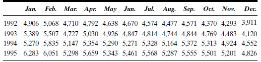
Glen Murphy was not happy to be chastised by his daughter. He decided to conduct an intensive search of Murphy Brothers' records. Upon implementing an investigation, he was excited to discover sales data for the past four years, 1992 through 1995, as shown in Table 3-9. He was surprised to find out that Julie did not share his enthusiasm. She knew that acquiring actual sales data for the past 4 years was a positive occurrence. Julie's problem was that she was not quite sure what to do with the newly acquired data.
TABLE 3-9 Monthly Sales for Murphy Brothers Furniture, 1992-1995

Source: Murphy Brothers sales records.
What should Julie conclude about Murphy Brothers' sales data?
Glen Murphy was not happy to be chastised by his daughter. He decided to conduct an intensive search of Murphy Brothers' records. Upon implementing an investigation, he was excited to discover sales data for the past four years, 1992 through 1995, as shown in Table 3-9. He was surprised to find out that Julie did not share his enthusiasm. She knew that acquiring actual sales data for the past 4 years was a positive occurrence. Julie's problem was that she was not quite sure what to do with the newly acquired data.
TABLE 3-9 Monthly Sales for Murphy Brothers Furniture, 1992-1995
Source: Murphy Brothers sales records.
What should Julie conclude about Murphy Brothers' sales data?
Question
MURPHY BROTHERS FURNITURE
Glen Murphy was not happy to be chastised by his daughter. He decided to conduct an intensive search of Murphy Brothers' records. Upon implementing an investigation, he was excited to discover sales data for the past four years, 1992 through 1995, as shown in Table 3-9. He was surprised to find out that Julie did not share his enthusiasm. She knew that acquiring actual sales data for the past 4 years was a positive occurrence. Julie's problem was that she was not quite sure what to do with the newly acquired data.
TABLE 3-9 Monthly Sales for Murphy Brothers Furniture, 1992-1995
Source: Murphy Brothers sales records.
How does the pattern of the actual sales data compare to the pattern of the retail sales data presented in Case 3-1A?
Question
MURPHY BROTHERS FURNITURE
Glen Murphy was not happy to be chastised by his daughter. He decided to conduct an intensive search of Murphy Brothers' records. Upon implementing an investigation, he was excited to discover sales data for the past four years, 1992 through 1995, as shown in Table 3-9. He was surprised to find out that Julie did not share his enthusiasm. She knew that acquiring actual sales data for the past 4 years was a positive occurrence. Julie's problem was that she was not quite sure what to do with the newly acquired data.
TABLE 3-9 Monthly Sales for Murphy Brothers Furniture, 1992-1995

Source: Murphy Brothers sales records.
Which data should Julie use to develop a forecasting model?
Glen Murphy was not happy to be chastised by his daughter. He decided to conduct an intensive search of Murphy Brothers' records. Upon implementing an investigation, he was excited to discover sales data for the past four years, 1992 through 1995, as shown in Table 3-9. He was surprised to find out that Julie did not share his enthusiasm. She knew that acquiring actual sales data for the past 4 years was a positive occurrence. Julie's problem was that she was not quite sure what to do with the newly acquired data.
TABLE 3-9 Monthly Sales for Murphy Brothers Furniture, 1992-1995
Source: Murphy Brothers sales records.
Which data should Julie use to develop a forecasting model?
Question
TUX
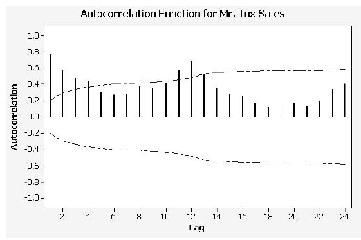
John Mosby, owner of several Mr. Tux rental stores, is beginning to forecast his most important business variable, monthly dollar sales (see the Mr. Tux cases at the ends of Chapters 1 and 2). One of his employees, Virginia Perot, has gathered the sales data shown in Case 2-2. John decides to use all 96 months of data he has collected. He runs the data on Minitab and obtains the autocorrelation function shown in Figure 3-25. Since all the autocorrelation coefficients are positive and they are trailing off very slowly, John concludes that his data have a trend.
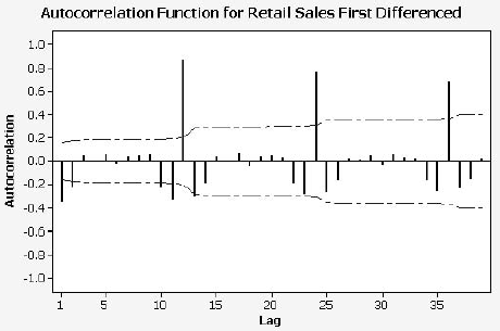
Next, John asks the program to compute the first differences of the data. Figure 3-26 shows the autocorrelation function for the differenced data. The autocorrelation coefficients for time lags 12 and 24, r 12 =.68 and r 24 =.42, respectively, are both significantly different from zero.
Finally, John uses another computer program to calculate the percentage of the variance in the original data explained by the trend, seasonal, and random components.
The program calculates the percentage of the variance in the original data explained by the factors in the analysis:

FIGURE 3-26 Autocorrelation Function for Mr. Tux Data First Differenced

Summarize the results of John's analysis in one paragraph that a manager, not a forecaster, can understand.
John Mosby, owner of several Mr. Tux rental stores, is beginning to forecast his most important business variable, monthly dollar sales (see the Mr. Tux cases at the ends of Chapters 1 and 2). One of his employees, Virginia Perot, has gathered the sales data shown in Case 2-2. John decides to use all 96 months of data he has collected. He runs the data on Minitab and obtains the autocorrelation function shown in Figure 3-25. Since all the autocorrelation coefficients are positive and they are trailing off very slowly, John concludes that his data have a trend.
Next, John asks the program to compute the first differences of the data. Figure 3-26 shows the autocorrelation function for the differenced data. The autocorrelation coefficients for time lags 12 and 24, r 12 =.68 and r 24 =.42, respectively, are both significantly different from zero.
Finally, John uses another computer program to calculate the percentage of the variance in the original data explained by the trend, seasonal, and random components.
The program calculates the percentage of the variance in the original data explained by the factors in the analysis:
FIGURE 3-26 Autocorrelation Function for Mr. Tux Data First Differenced
Summarize the results of John's analysis in one paragraph that a manager, not a forecaster, can understand.
Question
TUX
John Mosby, owner of several Mr. Tux rental stores, is beginning to forecast his most important business variable, monthly dollar sales (see the Mr. Tux cases at the ends of Chapters 1 and 2). One of his employees, Virginia Perot, has gathered the sales data shown in Case 2-2. John decides to use all 96 months of data he has collected. He runs the data on Minitab and obtains the autocorrelation function shown in Figure 3-25. Since all the autocorrelation coefficients are positive and they are trailing off very slowly, John concludes that his data have a trend.
Next, John asks the program to compute the first differences of the data. Figure 3-26 shows the autocorrelation function for the differenced data. The autocorrelation coefficients for time lags 12 and 24, r 12 =.68 and r 24 =.42, respectively, are both significantly different from zero.
Finally, John uses another computer program to calculate the percentage of the variance in the original data explained by the trend, seasonal, and random components.
The program calculates the percentage of the variance in the original data explained by the factors in the analysis:
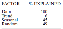
FIGURE 3-26 Autocorrelation Function for Mr. Tux Data First Differenced

Describe the trend and seasonal effects that appear to be present in the sales data for Mr. Tux.
John Mosby, owner of several Mr. Tux rental stores, is beginning to forecast his most important business variable, monthly dollar sales (see the Mr. Tux cases at the ends of Chapters 1 and 2). One of his employees, Virginia Perot, has gathered the sales data shown in Case 2-2. John decides to use all 96 months of data he has collected. He runs the data on Minitab and obtains the autocorrelation function shown in Figure 3-25. Since all the autocorrelation coefficients are positive and they are trailing off very slowly, John concludes that his data have a trend.
Next, John asks the program to compute the first differences of the data. Figure 3-26 shows the autocorrelation function for the differenced data. The autocorrelation coefficients for time lags 12 and 24, r 12 =.68 and r 24 =.42, respectively, are both significantly different from zero.
Finally, John uses another computer program to calculate the percentage of the variance in the original data explained by the trend, seasonal, and random components.
The program calculates the percentage of the variance in the original data explained by the factors in the analysis:
FIGURE 3-26 Autocorrelation Function for Mr. Tux Data First Differenced
Describe the trend and seasonal effects that appear to be present in the sales data for Mr. Tux.
Question
TUX
John Mosby, owner of several Mr. Tux rental stores, is beginning to forecast his most important business variable, monthly dollar sales (see the Mr. Tux cases at the ends of Chapters 1 and 2). One of his employees, Virginia Perot, has gathered the sales data shown in Case 2-2. John decides to use all 96 months of data he has collected. He runs the data on Minitab and obtains the autocorrelation function shown in Figure 3-25. Since all the autocorrelation coefficients are positive and they are trailing off very slowly, John concludes that his data have a trend.
Next, John asks the program to compute the first differences of the data. Figure 3-26 shows the autocorrelation function for the differenced data. The autocorrelation coefficients for time lags 12 and 24, r 12 =.68 and r 24 =.42, respectively, are both significantly different from zero.
Finally, John uses another computer program to calculate the percentage of the variance in the original data explained by the trend, seasonal, and random components.
The program calculates the percentage of the variance in the original data explained by the factors in the analysis:

FIGURE 3-26 Autocorrelation Function for Mr. Tux Data First Differenced
How would you explain the line "Random 49%."?
John Mosby, owner of several Mr. Tux rental stores, is beginning to forecast his most important business variable, monthly dollar sales (see the Mr. Tux cases at the ends of Chapters 1 and 2). One of his employees, Virginia Perot, has gathered the sales data shown in Case 2-2. John decides to use all 96 months of data he has collected. He runs the data on Minitab and obtains the autocorrelation function shown in Figure 3-25. Since all the autocorrelation coefficients are positive and they are trailing off very slowly, John concludes that his data have a trend.
Next, John asks the program to compute the first differences of the data. Figure 3-26 shows the autocorrelation function for the differenced data. The autocorrelation coefficients for time lags 12 and 24, r 12 =.68 and r 24 =.42, respectively, are both significantly different from zero.
Finally, John uses another computer program to calculate the percentage of the variance in the original data explained by the trend, seasonal, and random components.
The program calculates the percentage of the variance in the original data explained by the factors in the analysis:
FIGURE 3-26 Autocorrelation Function for Mr. Tux Data First Differenced
How would you explain the line "Random 49%."?
Question
TUX
John Mosby, owner of several Mr. Tux rental stores, is beginning to forecast his most important business variable, monthly dollar sales (see the Mr. Tux cases at the ends of Chapters 1 and 2). One of his employees, Virginia Perot, has gathered the sales data shown in Case 2-2. John decides to use all 96 months of data he has collected. He runs the data on Minitab and obtains the autocorrelation function shown in Figure 3-25. Since all the autocorrelation coefficients are positive and they are trailing off very slowly, John concludes that his data have a trend.
Next, John asks the program to compute the first differences of the data. Figure 3-26 shows the autocorrelation function for the differenced data. The autocorrelation coefficients for time lags 12 and 24, r 12 =.68 and r 24 =.42, respectively, are both significantly different from zero.
Finally, John uses another computer program to calculate the percentage of the variance in the original data explained by the trend, seasonal, and random components.
The program calculates the percentage of the variance in the original data explained by the factors in the analysis:

FIGURE 3-26 Autocorrelation Function for Mr. Tux Data First Differenced

Consider the significant autocorrelations, r 12 and r 24 , for the differenced data. Would you conclude that the sales first differenced have a seasonal component? If so, what are the implications for forecasting, say, the monthly changes in sales?
John Mosby, owner of several Mr. Tux rental stores, is beginning to forecast his most important business variable, monthly dollar sales (see the Mr. Tux cases at the ends of Chapters 1 and 2). One of his employees, Virginia Perot, has gathered the sales data shown in Case 2-2. John decides to use all 96 months of data he has collected. He runs the data on Minitab and obtains the autocorrelation function shown in Figure 3-25. Since all the autocorrelation coefficients are positive and they are trailing off very slowly, John concludes that his data have a trend.
Next, John asks the program to compute the first differences of the data. Figure 3-26 shows the autocorrelation function for the differenced data. The autocorrelation coefficients for time lags 12 and 24, r 12 =.68 and r 24 =.42, respectively, are both significantly different from zero.
Finally, John uses another computer program to calculate the percentage of the variance in the original data explained by the trend, seasonal, and random components.
The program calculates the percentage of the variance in the original data explained by the factors in the analysis:
FIGURE 3-26 Autocorrelation Function for Mr. Tux Data First Differenced
Consider the significant autocorrelations, r 12 and r 24 , for the differenced data. Would you conclude that the sales first differenced have a seasonal component? If so, what are the implications for forecasting, say, the monthly changes in sales?
Question
CONSUMER CREDIT COUNSELING
The Consumer Credit Counseling (CCC) operation was described in Case 1-2.
Marv Harnishfeger, executive director, was concerned about the size and scheduling of staff for the remainder of 1993. He explained the problem to Dorothy Mercer, recently elected president of the executive committee. Dorothy thought about the problem and concluded that CCC needed to analyze the number of new clients it acquired each month.
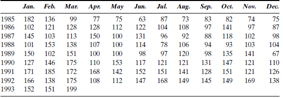
Dorothy, who worked for a local utility and was familiar with various data exploration techniques, agreed to analyze the problem. She asked Marv to provide monthly data for the number of new clients seen. Marv provided the monthly data shown in Table 3-10 for the number of new clients seen by CCC for the period January 1985 through March 1993. Dorothy then analyzed these data using a time series plot and autocorrelation analysis.
TABLE 3-10 Number of New Clients Seen by CCC from January 1985 through March 1993

Explain how Dorothy used autocorrelation analysis to explore the data pattern for the number of new clients seen by CCC.
The Consumer Credit Counseling (CCC) operation was described in Case 1-2.
Marv Harnishfeger, executive director, was concerned about the size and scheduling of staff for the remainder of 1993. He explained the problem to Dorothy Mercer, recently elected president of the executive committee. Dorothy thought about the problem and concluded that CCC needed to analyze the number of new clients it acquired each month.
Dorothy, who worked for a local utility and was familiar with various data exploration techniques, agreed to analyze the problem. She asked Marv to provide monthly data for the number of new clients seen. Marv provided the monthly data shown in Table 3-10 for the number of new clients seen by CCC for the period January 1985 through March 1993. Dorothy then analyzed these data using a time series plot and autocorrelation analysis.
TABLE 3-10 Number of New Clients Seen by CCC from January 1985 through March 1993
Explain how Dorothy used autocorrelation analysis to explore the data pattern for the number of new clients seen by CCC.
Question
CONSUMER CREDIT COUNSELING
The Consumer Credit Counseling (CCC) operation was described in Case 1-2.
Marv Harnishfeger, executive director, was concerned about the size and scheduling of staff for the remainder of 1993. He explained the problem to Dorothy Mercer, recently elected president of the executive committee. Dorothy thought about the problem and concluded that CCC needed to analyze the number of new clients it acquired each month.
Dorothy, who worked for a local utility and was familiar with various data exploration techniques, agreed to analyze the problem. She asked Marv to provide monthly data for the number of new clients seen. Marv provided the monthly data shown in Table 3-10 for the number of new clients seen by CCC for the period January 1985 through March 1993. Dorothy then analyzed these data using a time series plot and autocorrelation analysis.
TABLE 3-10 Number of New Clients Seen by CCC from January 1985 through March 1993

What did she conclude after she completed this analysis?
The Consumer Credit Counseling (CCC) operation was described in Case 1-2.
Marv Harnishfeger, executive director, was concerned about the size and scheduling of staff for the remainder of 1993. He explained the problem to Dorothy Mercer, recently elected president of the executive committee. Dorothy thought about the problem and concluded that CCC needed to analyze the number of new clients it acquired each month.
Dorothy, who worked for a local utility and was familiar with various data exploration techniques, agreed to analyze the problem. She asked Marv to provide monthly data for the number of new clients seen. Marv provided the monthly data shown in Table 3-10 for the number of new clients seen by CCC for the period January 1985 through March 1993. Dorothy then analyzed these data using a time series plot and autocorrelation analysis.
TABLE 3-10 Number of New Clients Seen by CCC from January 1985 through March 1993
What did she conclude after she completed this analysis?
Question
CONSUMER CREDIT COUNSELING
The Consumer Credit Counseling (CCC) operation was described in Case 1-2.
Marv Harnishfeger, executive director, was concerned about the size and scheduling of staff for the remainder of 1993. He explained the problem to Dorothy Mercer, recently elected president of the executive committee. Dorothy thought about the problem and concluded that CCC needed to analyze the number of new clients it acquired each month.
Dorothy, who worked for a local utility and was familiar with various data exploration techniques, agreed to analyze the problem. She asked Marv to provide monthly data for the number of new clients seen. Marv provided the monthly data shown in Table 3-10 for the number of new clients seen by CCC for the period January 1985 through March 1993. Dorothy then analyzed these data using a time series plot and autocorrelation analysis.
TABLE 3-10 Number of New Clients Seen by CCC from January 1985 through March 1993
What type of forecasting technique did Dorothy recommend for this data set?
Question
ALOMEGA FOOD STORES
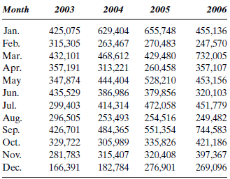
In Example 1.1, the president of Alomega, Julie Ruth, had collected data from her company's operations. She found several months of sales data along with several possible predictor variables (review this situation in Example 1.1). While her analysis team was working with the data in an attempt to forecast monthly sales, she became impatient and wondered which of the predictor variables was best for this purpose.
In Case 2-3, Julie investigated the relationships between sales and the possible predictor variables. She now realizes that this step was premature because she doesn't even know the data pattern of her sales. (See Table 3-11.)
TABLE 3-11 Monthly Sales for 27 Alomega Food Stores, 2003-2006
What did Julie conclude about the data pattern of Alomega Sales?
Question
SURTIDO COOKIES
GAMESA Company is the largest producer of cookies, snacks, and pastry in Mexico and Latin America.
Jame Luna, an analyst for SINTEC, which is an important supply-chain consulting firm based in Mexico, is working with GAMESA on an optimal vehicle routing and docking system for all the distribution centers in Mexico. Forecasts of the demand for GAMESA products will help to produce a plan for the truck float and warehouse requirements associated with the optimal vehicle routing and docking system.
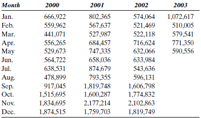
As a starting point, Jame decides to focus on one of the main products of the Cookies Division of GAMESA. He collects data on monthly aggregated demand (in kilograms) for Surtido cookies from January 2000 through May 2003. The results are shown in Table 3-12.
Surtido is a mixture of different cookies in one presentation. Jame knows that this product is commonly served at meetings, parties, and reunions. It is also popular during the Christmas holidays. So Jame is pretty sure there will be a seasonal component in the time series of monthly sales, but he is not sure if there is a trend in sales. He decides to plot the sales series and use autocorrelation analysis to help him determine if these data have a trend and a seasonal component.
Karin, one of the members of Jame's team, suggests that forecasts of future monthly sales might be generated by simply using the average sales for each month. Jame decides to test this suggestion by "holding out" the monthly sales for 2003 as test cases. Then the average of the January sales for 2000-2002 will be used to forecast January sales for 2003 and so forth.
TABLE 3-12 Monthly Sales (in kgs) for Surtido Cookies, January 2000-May 2003

What should Jame conclude about the data pattern of Surtido cookie sales?
GAMESA Company is the largest producer of cookies, snacks, and pastry in Mexico and Latin America.
Jame Luna, an analyst for SINTEC, which is an important supply-chain consulting firm based in Mexico, is working with GAMESA on an optimal vehicle routing and docking system for all the distribution centers in Mexico. Forecasts of the demand for GAMESA products will help to produce a plan for the truck float and warehouse requirements associated with the optimal vehicle routing and docking system.
As a starting point, Jame decides to focus on one of the main products of the Cookies Division of GAMESA. He collects data on monthly aggregated demand (in kilograms) for Surtido cookies from January 2000 through May 2003. The results are shown in Table 3-12.
Surtido is a mixture of different cookies in one presentation. Jame knows that this product is commonly served at meetings, parties, and reunions. It is also popular during the Christmas holidays. So Jame is pretty sure there will be a seasonal component in the time series of monthly sales, but he is not sure if there is a trend in sales. He decides to plot the sales series and use autocorrelation analysis to help him determine if these data have a trend and a seasonal component.
Karin, one of the members of Jame's team, suggests that forecasts of future monthly sales might be generated by simply using the average sales for each month. Jame decides to test this suggestion by "holding out" the monthly sales for 2003 as test cases. Then the average of the January sales for 2000-2002 will be used to forecast January sales for 2003 and so forth.
TABLE 3-12 Monthly Sales (in kgs) for Surtido Cookies, January 2000-May 2003
What should Jame conclude about the data pattern of Surtido cookie sales?
Question
SURTIDO COOKIES
GAMESA Company is the largest producer of cookies, snacks, and pastry in Mexico and Latin America.
Jame Luna, an analyst for SINTEC, which is an important supply-chain consulting firm based in Mexico, is working with GAMESA on an optimal vehicle routing and docking system for all the distribution centers in Mexico. Forecasts of the demand for GAMESA products will help to produce a plan for the truck float and warehouse requirements associated with the optimal vehicle routing and docking system.
As a starting point, Jame decides to focus on one of the main products of the Cookies Division of GAMESA. He collects data on monthly aggregated demand (in kilograms) for Surtido cookies from January 2000 through May 2003. The results are shown in Table 3-12.
Surtido is a mixture of different cookies in one presentation. Jame knows that this product is commonly served at meetings, parties, and reunions. It is also popular during the Christmas holidays. So Jame is pretty sure there will be a seasonal component in the time series of monthly sales, but he is not sure if there is a trend in sales. He decides to plot the sales series and use autocorrelation analysis to help him determine if these data have a trend and a seasonal component.
Karin, one of the members of Jame's team, suggests that forecasts of future monthly sales might be generated by simply using the average sales for each month. Jame decides to test this suggestion by "holding out" the monthly sales for 2003 as test cases. Then the average of the January sales for 2000-2002 will be used to forecast January sales for 2003 and so forth.
TABLE 3-12 Monthly Sales (in kgs) for Surtido Cookies, January 2000-May 2003
What did Jame learn about the forecast accuracy of Karin's suggestion?

Unlock Deck
Sign up to unlock the cards in this deck!
Unlock Deck
Unlock Deck
1/42
Play
Full screen (f)
Deck 2: Exploring Data Patterns and Choosing a Forecasting Technique
1
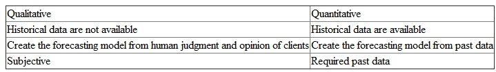
Explain the differences between qualitative and quantitative forecasting techniques.
Qualitative forecasting techniques:
The qualitative forecasting technique depends on human judgment and examination of clients with the ranking scale which are subjective. In other words, prior data is not available. The qualitative forecasting techniques are listed below:
• Executive opinions
• Delphi technique
• Sales force pooling
• Consumes surveys
Quantitative forecasting techniques:
The above technique forecast the future data when past data is available. This method is based on the historical data. The quantitative forecasting techniques are listed below:
• Naive methods
• Moving average methods
• Exponential smoothing average methods
• Trend analysis
• Decomposition of time series
Differences between qualitative and quantitative forecasting techniques are tabulated below:
2
What is a time series?
Time series:
The data that are collected, recorded, or observed over successive increments of time is termed as time series. In other words, the time series is calculated over a time interval. That is, the data, which can be measured in year, week, month etc, is a time series data. Moreover, the time-series plot explains how the value of a variable has changed over time.
The data that are collected, recorded, or observed over successive increments of time is termed as time series. In other words, the time series is calculated over a time interval. That is, the data, which can be measured in year, week, month etc, is a time series data. Moreover, the time-series plot explains how the value of a variable has changed over time.
3
Describe each of the components in a time series.
The components of the time series model are,
• Trend component
• Cyclical component
• Irregular component
• Seasonal component
Trend component indicates the overall long term upward or downward pattern of tendency in the time series.
The cyclical component shows the repeating up and down movements through all phases of the time series.
Irregular component data do not follow the trend modified by the cyclic components and the data have only random fluctuations in the series.
When the data have periodic fluctuations and that data are recorded monthly or quarterly, then the time series represents Seasonal component.
4
What is autocorrelation?
Unlock Deck
Unlock for access to all 42 flashcards in this deck.
Unlock Deck
k this deck
5
What does an autocorrelation coefficient measure?
Unlock Deck
Unlock for access to all 42 flashcards in this deck.
Unlock Deck
k this deck
6
Describe how correlograms are used to analyze autocorrelations for various lags of a time series.
Unlock Deck
Unlock for access to all 42 flashcards in this deck.
Unlock Deck
k this deck
7
Indicate whether each of the following statements describes a stationary or a non-stationary series.
a. A series that has a trend
b. A series whose mean and variance remain constant over time
c. A series whose mean value is changing over time
d. A series that contains no growth or decline
a. A series that has a trend
b. A series whose mean and variance remain constant over time
c. A series whose mean value is changing over time
d. A series that contains no growth or decline
Unlock Deck
Unlock for access to all 42 flashcards in this deck.
Unlock Deck
k this deck
8
Descriptions are provided for several types of series: random, stationary, trending, and seasonal. Identify the type of series that each describes.
a. The series has basic statistical properties, such as the mean and variance, that remain constant over time.
b. The successive values of a time series are not related to each other.
c. A high relationship exists between each successive value of a series.
d. A significant autocorrelation coefficient appears at time lag 4 for quarterly data.
e. The series contains no growth or decline.
f. The autocorrelation coefficients are typically significantly different from zero for the first several time lags and then gradually decrease toward zero as the number of lags increases.
Unlock Deck
Unlock for access to all 42 flashcards in this deck.
Unlock Deck
k this deck
9
List some of the forecasting techniques that should be considered when forecasting a stationary series. Give examples of situations in which these techniques would be applicable.
Unlock Deck
Unlock for access to all 42 flashcards in this deck.
Unlock Deck
k this deck
10
List some of the forecasting techniques that should be considered when forecasting a trending series. Give examples of situations in which these techniques would be applicable.
Unlock Deck
Unlock for access to all 42 flashcards in this deck.
Unlock Deck
k this deck
11
List some of the forecasting techniques that should be considered when forecasting a seasonal series. Give examples of situations in which these techniques would be applicable.
Unlock Deck
Unlock for access to all 42 flashcards in this deck.
Unlock Deck
k this deck
12
List some of the forecasting techniques that should be considered when forecasting a cyclical series. Give examples of situations in which these techniques would be applicable.
Unlock Deck
Unlock for access to all 42 flashcards in this deck.
Unlock Deck
k this deck
13
The number of marriages in the United States is given in Table P-13. Compute the first differences for these data. Plot the original data and the difference data as a time series. Is there a trend in either of these series? Discuss.
TABLE P-13
Source: Based on Statistical Abstract of the United States, various years.
TABLE P-13
Source: Based on Statistical Abstract of the United States, various years.
Unlock Deck
Unlock for access to all 42 flashcards in this deck.
Unlock Deck
k this deck
14
Compute the 95% confidence interval for the autocorrelation coefficient for time lag 1 for a series that contains 80 terms.
Unlock Deck
Unlock for access to all 42 flashcards in this deck.
Unlock Deck
k this deck
15
Which measure of forecast accuracy should be used in each of the following situations?
a. The analyst needs to determine whether a forecasting method is biased.
b. The analyst feels that the size or magnitude of the forecast variable is important in evaluating the accuracy of the forecast.
c. The analyst needs to penalize large forecasting errors.
a. The analyst needs to determine whether a forecasting method is biased.
b. The analyst feels that the size or magnitude of the forecast variable is important in evaluating the accuracy of the forecast.
c. The analyst needs to penalize large forecasting errors.
Unlock Deck
Unlock for access to all 42 flashcards in this deck.
Unlock Deck
k this deck
16
Which of the following statements is true concerning the accuracy measures used to evaluate forecasts?
a. The MAPE takes into consideration the magnitude of the values being forecast.
b. The MSE and RMSE penalize large errors.
c. The MPE is used to determine whether a model is systematically predicting too high or too low.
d. The advantage of the MAD method is that it relates the size of the error to the actual observation.
Unlock Deck
Unlock for access to all 42 flashcards in this deck.
Unlock Deck
k this deck
17
Allie White, the chief loan officer for the Dominion Bank, would like to analyze the bank's loan portfolio for the years 2001 to 2006. The data are shown in Table P-17.
a. Compute the autocorrelations for time lags 1 and 2. Test to determine whether these autocorrelation coefficients are significantly different from zero at the.05 significance level.
b. Use a computer program to plot the data and compute the autocorrelations for the first six time lags. Is this time series stationary?
TABLE P-17 Quarterly Loans ($ millions) for Dominion Bank, 2001-2006
Source: Based on Dominion Bank records.
Unlock Deck
Unlock for access to all 42 flashcards in this deck.
Unlock Deck
k this deck
18
This question refers to Problem 17. Compute the first differences of the quarterly loan data for Dominion Bank.
a. Compute the autocorrelation coefficient for time lag 1 using the differenced data.
b. Use a computer program to plot the differenced data and compute the autocorrelations for the differenced data for the first six time lags. Is this time series stationary?
a. Compute the autocorrelation coefficient for time lag 1 using the differenced data.
b. Use a computer program to plot the differenced data and compute the autocorrelations for the differenced data for the first six time lags. Is this time series stationary?
Unlock Deck
Unlock for access to all 42 flashcards in this deck.
Unlock Deck
k this deck
19
Analyze the autocorrelation coefficients for the series shown in Figures 3-18 through 3-21. Briefly describe each series.
FIGURE 3-18 Autocorrelation Function
FIGURE 3-19 Autocorrelation Function
FIGURE 3-20 Autocorrelation Function
FIGURE 3-21 Autocorrelation Function
FIGURE 3-18 Autocorrelation Function
FIGURE 3-19 Autocorrelation Function
FIGURE 3-20 Autocorrelation Function
FIGURE 3-21 Autocorrelation Function
Unlock Deck
Unlock for access to all 42 flashcards in this deck.
Unlock Deck
k this deck
20
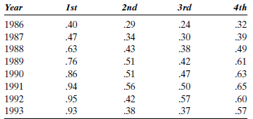
An analyst would like to determine whether there is a pattern to earnings per share for the Price Company, which operated a wholesale/retail cash-and-carry business in several states under the name Price Club. The data are shown in Table P-20. Describe any patterns that exist in these data.
a. Find the forecast value of the quarterly earnings per share for Price Club for each quarter by using the naive approach (i.e., the forecast for first-quarter 1987 is the value for fourth-quarter 1986,.32).
b. Evaluate the naive forecast using MAD.
c. Evaluate the naive forecast using MSE and RMSE.
d. Evaluate the naive forecast using MAPE.
e. Evaluate the naive forecast using MPE.
TABLE P-20 Quarterly Earnings per Share for Price Club: 1986-1993 Quarter
Source: The Value Line Investment Survey (New York: Value Line, 1994), p. 1646.
a. Find the forecast value of the quarterly earnings per share for Price Club for each quarter by using the naive approach (i.e., the forecast for first-quarter 1987 is the value for fourth-quarter 1986,.32).
b. Evaluate the naive forecast using MAD.
c. Evaluate the naive forecast using MSE and RMSE.
d. Evaluate the naive forecast using MAPE.
e. Evaluate the naive forecast using MPE.
TABLE P-20 Quarterly Earnings per Share for Price Club: 1986-1993 Quarter
Source: The Value Line Investment Survey (New York: Value Line, 1994), p. 1646.
Unlock Deck
Unlock for access to all 42 flashcards in this deck.
Unlock Deck
k this deck
21
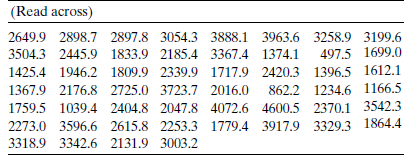
Table P-21 contains the weekly sales for a food item for 52 consecutive weeks.
a. Plot the sales data as a time series.
b. Do you think this series is stationary or nonstationary?
c. Using Minitab or a similar program, compute the autocorrelations of the sales series for the first 10 time lags. Is the behavior of the autocorrelations consistent with your choice in part b? Explain.
TABLE P-21 Weekly Sales of a Food Item
a. Plot the sales data as a time series.
b. Do you think this series is stationary or nonstationary?
c. Using Minitab or a similar program, compute the autocorrelations of the sales series for the first 10 time lags. Is the behavior of the autocorrelations consistent with your choice in part b? Explain.
TABLE P-21 Weekly Sales of a Food Item
Unlock Deck
Unlock for access to all 42 flashcards in this deck.
Unlock Deck
k this deck
22
This question refers to Problem 21.
a. Fit the random model given by Equation 3.4 to the data in Table P-21 by estimating c with the sample mean
so
. Compute the residuals using
.
b. Using Minitab or a similar program, compute the autocorrelations of the residuals from part c for the first 10 time lags. Is the random model adequate for the sales data? Explain.
TABLE P-21 Weekly Sales of a Food Item
a. Fit the random model given by Equation 3.4 to the data in Table P-21 by estimating c with the sample mean
so . Compute the residuals using .b. Using Minitab or a similar program, compute the autocorrelations of the residuals from part c for the first 10 time lags. Is the random model adequate for the sales data? Explain.
TABLE P-21 Weekly Sales of a Food Item
Unlock Deck
Unlock for access to all 42 flashcards in this deck.
Unlock Deck
k this deck
23
Table P-23 contains Southwest Airlines' quarterly income before extraordinary items ($MM) for the years 1988-1999.
a. Plot the income data as a time series and describe any patterns that exist.
b. Is this series stationary or nonstationary? Explain.
c. Using Minitab or a similar program, compute the autocorrelations of the income series for the first 10 time lags. Is the behavior of the autocorrelations consistent with your choice in part b? Explain.
TABLE P-23 Quarterly Income for Southwest Airlines ($MM)
Source: Based on Compustat Industrial Quarterly Data Base
Unlock Deck
Unlock for access to all 42 flashcards in this deck.
Unlock Deck
k this deck
24
This question refers to Problem 23.
a. Use Minitab or Excel to compute the fourth differences of the income data in Table P-23. Fourth differences are computed by differencing observations four time periods apart. With quarterly data, this procedure is sometimes useful for creating a stationary series from a nonstationary series (see Chapter 9). Consequently, the fourth differenced data will be Y 5 ? Y 1 = 19.64 ?.17 = 19.47, Y 6 ? Y 2 = 19.24 ? 15.13 = 4.11,... , and so forth.
b. Plot the time series of fourth differences. Does this time series appear to be stationary or nonstationary? Explain.
TABLE P-23 Quarterly Income for Southwest Airlines ($MM)
Source: Based on Compustat Industrial Quarterly Data Base
Unlock Deck
Unlock for access to all 42 flashcards in this deck.
Unlock Deck
k this deck
25
This question refers to Problem 23.
TABLE P-23 Quarterly Income for Southwest Airlines ($MM)
Source: Based on Compustat Industrial Quarterly Data Base.
a. Consider a naive forecasting method where the first-quarter income is used to forecast first-quarter income for the following year, second-quarter income is used to forecast second-quarter income, and so forth. For example, a forecast of first-quarter income for 1998 is provided by the first-quarter income for 1997, 50.87 (see Table P-23). Use this naive method to calculate forecasts of quarterly income for the years 1998-1999.
b. Using the forecasts in part a, calculate the MAD, RMSE, and MAPE.
c. Given the results in part b and the nature of the patterns in the income series, do you think this naive forecasting method is viable? Can you think of another naive method that might be better?
Unlock Deck
Unlock for access to all 42 flashcards in this deck.
Unlock Deck
k this deck
26
MURPHY BROTHERS FURNITURE
In 1958, the Murphy brothers established a furniture store in downtown Dallas. Over the years, they were quite successful and extended their retail coverage throughout the West and Midwest. By 1996, their chain of furniture stores had become well established in 36 states.
Julie Murphy, the daughter of one of the founders, had recently joined the firm. Her father and uncle were sophisticated in many ways but not in the area of quantitative skills. In particular, they both felt that they could not accurately forecast the future sales of Murphy Brothers using modern computer techniques. For this reason, they appealed to Julie for help as part of her new job.
Julie first considered using Murphy sales dollars as her variable but found that several years of history were missing. She asked her father, Glen, about this, and he told her that at the time he "didn't think it was that important." Julie explained the importance of past data to Glen, and he indicated that he would save future data.
Julie decided that Murphy sales were probably closely related to national sales figures and decided to search for an appropriate variable in one of the many federal publications. After looking through a recent copy of the Survey of Current Business, she found the history on monthly sales for all retail stores in the United States and decided to use this variable as a substitute for her variable of interest, Murphy Brothers sales dollars. She reasoned that, if she could establish accurate forecasts for national sales, she could relate these forecasts to Murphy's own sales and come up with the forecasts she wanted.
Table 3-8 shows the data that Julie collected, and Figure 3-22 shows a data plot provided by Julie's computer program. Julie began her analysis by using the computer to develop a plot of the autocorrelation coefficients.
After examining the autocorrelation function produced in Figure 3-23, it was obvious to Julie that her data contain a trend. The early autocorrelation coefficients are very large, and they drop toward zero very slowly with time. To make the series stationary so that various forecasting methods could be considered, Julie decided to first difference her data to see if the trend could be removed. The autocorrelation function for the first differenced data is shown in Figure 3-24.
TABLE 3-8 Monthly Sales ($ billions) for All Retail Stores, 1983-1995
Source: Based on Survey of Current Business , various years.
FIGURE 3-22 Time Series Graph of Monthly Sales for All U.S. Retail Stores, 1983-1995
FIGURE 3-23 Autocorrelation Function for Monthly Sales for All U.S. Retail Stores
FIGURE 3-24 Autocorrelation Function for Monthly Sales for All U.S. Retail Stores First Differenced
What should Julie conclude about the retail sales series?
Unlock Deck
Unlock for access to all 42 flashcards in this deck.
Unlock Deck
k this deck
27
MURPHY BROTHERS FURNITURE
In 1958, the Murphy brothers established a furniture store in downtown Dallas. Over the years, they were quite successful and extended their retail coverage throughout the West and Midwest. By 1996, their chain of furniture stores had become well established in 36 states.
Julie Murphy, the daughter of one of the founders, had recently joined the firm. Her father and uncle were sophisticated in many ways but not in the area of quantitative skills. In particular, they both felt that they could not accurately forecast the future sales of Murphy Brothers using modern computer techniques. For this reason, they appealed to Julie for help as part of her new job.
Julie first considered using Murphy sales dollars as her variable but found that several years of history were missing. She asked her father, Glen, about this, and he told her that at the time he "didn't think it was that important." Julie explained the importance of past data to Glen, and he indicated that he would save future data.
Julie decided that Murphy sales were probably closely related to national sales figures and decided to search for an appropriate variable in one of the many federal publications. After looking through a recent copy of the Survey of Current Business, she found the history on monthly sales for all retail stores in the United States and decided to use this variable as a substitute for her variable of interest, Murphy Brothers sales dollars. She reasoned that, if she could establish accurate forecasts for national sales, she could relate these forecasts to Murphy's own sales and come up with the forecasts she wanted.
Table 3-8 shows the data that Julie collected, and Figure 3-22 shows a data plot provided by Julie's computer program. Julie began her analysis by using the computer to develop a plot of the autocorrelation coefficients.
After examining the autocorrelation function produced in Figure 3-23, it was obvious to Julie that her data contain a trend. The early autocorrelation coefficients are very large, and they drop toward zero very slowly with time. To make the series stationary so that various forecasting methods could be considered, Julie decided to first difference her data to see if the trend could be removed. The autocorrelation function for the first differenced data is shown in Figure 3-24.
TABLE 3-8 Monthly Sales ($ billions) for All Retail Stores, 1983-1995
Source: Based on Survey of Current Business , various years.
FIGURE 3-22 Time Series Graph of Monthly Sales for All U.S. Retail Stores, 1983-1995
FIGURE 3-23 Autocorrelation Function for Monthly Sales for All U.S. Retail Stores
FIGURE 3-24 Autocorrelation Function for Monthly Sales for All U.S. Retail Stores First Differenced
Has Julie made good progress toward finding a forecasting technique?
Unlock Deck
Unlock for access to all 42 flashcards in this deck.
Unlock Deck
k this deck
28
MURPHY BROTHERS FURNITURE
In 1958, the Murphy brothers established a furniture store in downtown Dallas. Over the years, they were quite successful and extended their retail coverage throughout the West and Midwest. By 1996, their chain of furniture stores had become well established in 36 states.
Julie Murphy, the daughter of one of the founders, had recently joined the firm. Her father and uncle were sophisticated in many ways but not in the area of quantitative skills. In particular, they both felt that they could not accurately forecast the future sales of Murphy Brothers using modern computer techniques. For this reason, they appealed to Julie for help as part of her new job.
Julie first considered using Murphy sales dollars as her variable but found that several years of history were missing. She asked her father, Glen, about this, and he told her that at the time he "didn't think it was that important." Julie explained the importance of past data to Glen, and he indicated that he would save future data.
Julie decided that Murphy sales were probably closely related to national sales figures and decided to search for an appropriate variable in one of the many federal publications. After looking through a recent copy of the Survey of Current Business, she found the history on monthly sales for all retail stores in the United States and decided to use this variable as a substitute for her variable of interest, Murphy Brothers sales dollars. She reasoned that, if she could establish accurate forecasts for national sales, she could relate these forecasts to Murphy's own sales and come up with the forecasts she wanted.
Table 3-8 shows the data that Julie collected, and Figure 3-22 shows a data plot provided by Julie's computer program. Julie began her analysis by using the computer to develop a plot of the autocorrelation coefficients.
After examining the autocorrelation function produced in Figure 3-23, it was obvious to Julie that her data contain a trend. The early autocorrelation coefficients are very large, and they drop toward zero very slowly with time. To make the series stationary so that various forecasting methods could be considered, Julie decided to first difference her data to see if the trend could be removed. The autocorrelation function for the first differenced data is shown in Figure 3-24.
TABLE 3-8 Monthly Sales ($ billions) for All Retail Stores, 1983-1995
Source: Based on Survey of Current Business , various years.
FIGURE 3-22 Time Series Graph of Monthly Sales for All U.S. Retail Stores, 1983-1995
FIGURE 3-23 Autocorrelation Function for Monthly Sales for All U.S. Retail Stores
FIGURE 3-24 Autocorrelation Function for Monthly Sales for All U.S. Retail Stores First Differenced
What forecasting techniques should Julie try?
Unlock Deck
Unlock for access to all 42 flashcards in this deck.
Unlock Deck
k this deck
29
MURPHY BROTHERS FURNITURE
In 1958, the Murphy brothers established a furniture store in downtown Dallas. Over the years, they were quite successful and extended their retail coverage throughout the West and Midwest. By 1996, their chain of furniture stores had become well established in 36 states.
Julie Murphy, the daughter of one of the founders, had recently joined the firm. Her father and uncle were sophisticated in many ways but not in the area of quantitative skills. In particular, they both felt that they could not accurately forecast the future sales of Murphy Brothers using modern computer techniques. For this reason, they appealed to Julie for help as part of her new job.
Julie first considered using Murphy sales dollars as her variable but found that several years of history were missing. She asked her father, Glen, about this, and he told her that at the time he "didn't think it was that important." Julie explained the importance of past data to Glen, and he indicated that he would save future data.
Julie decided that Murphy sales were probably closely related to national sales figures and decided to search for an appropriate variable in one of the many federal publications. After looking through a recent copy of the Survey of Current Business, she found the history on monthly sales for all retail stores in the United States and decided to use this variable as a substitute for her variable of interest, Murphy Brothers sales dollars. She reasoned that, if she could establish accurate forecasts for national sales, she could relate these forecasts to Murphy's own sales and come up with the forecasts she wanted.
Table 3-8 shows the data that Julie collected, and Figure 3-22 shows a data plot provided by Julie's computer program. Julie began her analysis by using the computer to develop a plot of the autocorrelation coefficients.
After examining the autocorrelation function produced in Figure 3-23, it was obvious to Julie that her data contain a trend. The early autocorrelation coefficients are very large, and they drop toward zero very slowly with time. To make the series stationary so that various forecasting methods could be considered, Julie decided to first difference her data to see if the trend could be removed. The autocorrelation function for the first differenced data is shown in Figure 3-24.
TABLE 3-8 Monthly Sales ($ billions) for All Retail Stores, 1983-1995
Source: Based on Survey of Current Business , various years.
FIGURE 3-22 Time Series Graph of Monthly Sales for All U.S. Retail Stores, 1983-1995
FIGURE 3-23 Autocorrelation Function for Monthly Sales for All U.S. Retail Stores
FIGURE 3-24 Autocorrelation Function for Monthly Sales for All U.S. Retail Stores First Differenced
How will Julie know which technique works best?
Unlock Deck
Unlock for access to all 42 flashcards in this deck.
Unlock Deck
k this deck
30
MURPHY BROTHERS FURNITURE
Glen Murphy was not happy to be chastised by his daughter. He decided to conduct an intensive search of Murphy Brothers' records. Upon implementing an investigation, he was excited to discover sales data for the past four years, 1992 through 1995, as shown in Table 3-9. He was surprised to find out that Julie did not share his enthusiasm. She knew that acquiring actual sales data for the past 4 years was a positive occurrence. Julie's problem was that she was not quite sure what to do with the newly acquired data.
TABLE 3-9 Monthly Sales for Murphy Brothers Furniture, 1992-1995
Source: Murphy Brothers sales records.
What should Julie conclude about Murphy Brothers' sales data?
Unlock Deck
Unlock for access to all 42 flashcards in this deck.
Unlock Deck
k this deck
31
MURPHY BROTHERS FURNITURE
Glen Murphy was not happy to be chastised by his daughter. He decided to conduct an intensive search of Murphy Brothers' records. Upon implementing an investigation, he was excited to discover sales data for the past four years, 1992 through 1995, as shown in Table 3-9. He was surprised to find out that Julie did not share his enthusiasm. She knew that acquiring actual sales data for the past 4 years was a positive occurrence. Julie's problem was that she was not quite sure what to do with the newly acquired data.
TABLE 3-9 Monthly Sales for Murphy Brothers Furniture, 1992-1995
Source: Murphy Brothers sales records.
How does the pattern of the actual sales data compare to the pattern of the retail sales data presented in Case 3-1A?
Unlock Deck
Unlock for access to all 42 flashcards in this deck.
Unlock Deck
k this deck
32
MURPHY BROTHERS FURNITURE
Glen Murphy was not happy to be chastised by his daughter. He decided to conduct an intensive search of Murphy Brothers' records. Upon implementing an investigation, he was excited to discover sales data for the past four years, 1992 through 1995, as shown in Table 3-9. He was surprised to find out that Julie did not share his enthusiasm. She knew that acquiring actual sales data for the past 4 years was a positive occurrence. Julie's problem was that she was not quite sure what to do with the newly acquired data.
TABLE 3-9 Monthly Sales for Murphy Brothers Furniture, 1992-1995
Source: Murphy Brothers sales records.
Which data should Julie use to develop a forecasting model?
Unlock Deck
Unlock for access to all 42 flashcards in this deck.
Unlock Deck
k this deck
33
TUX
John Mosby, owner of several Mr. Tux rental stores, is beginning to forecast his most important business variable, monthly dollar sales (see the Mr. Tux cases at the ends of Chapters 1 and 2). One of his employees, Virginia Perot, has gathered the sales data shown in Case 2-2. John decides to use all 96 months of data he has collected. He runs the data on Minitab and obtains the autocorrelation function shown in Figure 3-25. Since all the autocorrelation coefficients are positive and they are trailing off very slowly, John concludes that his data have a trend.
Next, John asks the program to compute the first differences of the data. Figure 3-26 shows the autocorrelation function for the differenced data. The autocorrelation coefficients for time lags 12 and 24, r 12 =.68 and r 24 =.42, respectively, are both significantly different from zero.
Finally, John uses another computer program to calculate the percentage of the variance in the original data explained by the trend, seasonal, and random components.
The program calculates the percentage of the variance in the original data explained by the factors in the analysis:
FIGURE 3-26 Autocorrelation Function for Mr. Tux Data First Differenced
Summarize the results of John's analysis in one paragraph that a manager, not a forecaster, can understand.
Unlock Deck
Unlock for access to all 42 flashcards in this deck.
Unlock Deck
k this deck
34
TUX
John Mosby, owner of several Mr. Tux rental stores, is beginning to forecast his most important business variable, monthly dollar sales (see the Mr. Tux cases at the ends of Chapters 1 and 2). One of his employees, Virginia Perot, has gathered the sales data shown in Case 2-2. John decides to use all 96 months of data he has collected. He runs the data on Minitab and obtains the autocorrelation function shown in Figure 3-25. Since all the autocorrelation coefficients are positive and they are trailing off very slowly, John concludes that his data have a trend.
Next, John asks the program to compute the first differences of the data. Figure 3-26 shows the autocorrelation function for the differenced data. The autocorrelation coefficients for time lags 12 and 24, r 12 =.68 and r 24 =.42, respectively, are both significantly different from zero.
Finally, John uses another computer program to calculate the percentage of the variance in the original data explained by the trend, seasonal, and random components.
The program calculates the percentage of the variance in the original data explained by the factors in the analysis:
FIGURE 3-26 Autocorrelation Function for Mr. Tux Data First Differenced
Describe the trend and seasonal effects that appear to be present in the sales data for Mr. Tux.
Unlock Deck
Unlock for access to all 42 flashcards in this deck.
Unlock Deck
k this deck
35
TUX
John Mosby, owner of several Mr. Tux rental stores, is beginning to forecast his most important business variable, monthly dollar sales (see the Mr. Tux cases at the ends of Chapters 1 and 2). One of his employees, Virginia Perot, has gathered the sales data shown in Case 2-2. John decides to use all 96 months of data he has collected. He runs the data on Minitab and obtains the autocorrelation function shown in Figure 3-25. Since all the autocorrelation coefficients are positive and they are trailing off very slowly, John concludes that his data have a trend.
Next, John asks the program to compute the first differences of the data. Figure 3-26 shows the autocorrelation function for the differenced data. The autocorrelation coefficients for time lags 12 and 24, r 12 =.68 and r 24 =.42, respectively, are both significantly different from zero.
Finally, John uses another computer program to calculate the percentage of the variance in the original data explained by the trend, seasonal, and random components.
The program calculates the percentage of the variance in the original data explained by the factors in the analysis:
FIGURE 3-26 Autocorrelation Function for Mr. Tux Data First Differenced
How would you explain the line "Random 49%."?
Unlock Deck
Unlock for access to all 42 flashcards in this deck.
Unlock Deck
k this deck
36
TUX
John Mosby, owner of several Mr. Tux rental stores, is beginning to forecast his most important business variable, monthly dollar sales (see the Mr. Tux cases at the ends of Chapters 1 and 2). One of his employees, Virginia Perot, has gathered the sales data shown in Case 2-2. John decides to use all 96 months of data he has collected. He runs the data on Minitab and obtains the autocorrelation function shown in Figure 3-25. Since all the autocorrelation coefficients are positive and they are trailing off very slowly, John concludes that his data have a trend.
Next, John asks the program to compute the first differences of the data. Figure 3-26 shows the autocorrelation function for the differenced data. The autocorrelation coefficients for time lags 12 and 24, r 12 =.68 and r 24 =.42, respectively, are both significantly different from zero.
Finally, John uses another computer program to calculate the percentage of the variance in the original data explained by the trend, seasonal, and random components.
The program calculates the percentage of the variance in the original data explained by the factors in the analysis:
FIGURE 3-26 Autocorrelation Function for Mr. Tux Data First Differenced
Consider the significant autocorrelations, r 12 and r 24 , for the differenced data. Would you conclude that the sales first differenced have a seasonal component? If so, what are the implications for forecasting, say, the monthly changes in sales?
Unlock Deck
Unlock for access to all 42 flashcards in this deck.
Unlock Deck
k this deck
37
CONSUMER CREDIT COUNSELING
The Consumer Credit Counseling (CCC) operation was described in Case 1-2.
Marv Harnishfeger, executive director, was concerned about the size and scheduling of staff for the remainder of 1993. He explained the problem to Dorothy Mercer, recently elected president of the executive committee. Dorothy thought about the problem and concluded that CCC needed to analyze the number of new clients it acquired each month.
Dorothy, who worked for a local utility and was familiar with various data exploration techniques, agreed to analyze the problem. She asked Marv to provide monthly data for the number of new clients seen. Marv provided the monthly data shown in Table 3-10 for the number of new clients seen by CCC for the period January 1985 through March 1993. Dorothy then analyzed these data using a time series plot and autocorrelation analysis.
TABLE 3-10 Number of New Clients Seen by CCC from January 1985 through March 1993
Explain how Dorothy used autocorrelation analysis to explore the data pattern for the number of new clients seen by CCC.
Unlock Deck
Unlock for access to all 42 flashcards in this deck.
Unlock Deck
k this deck
38
CONSUMER CREDIT COUNSELING
The Consumer Credit Counseling (CCC) operation was described in Case 1-2.
Marv Harnishfeger, executive director, was concerned about the size and scheduling of staff for the remainder of 1993. He explained the problem to Dorothy Mercer, recently elected president of the executive committee. Dorothy thought about the problem and concluded that CCC needed to analyze the number of new clients it acquired each month.
Dorothy, who worked for a local utility and was familiar with various data exploration techniques, agreed to analyze the problem. She asked Marv to provide monthly data for the number of new clients seen. Marv provided the monthly data shown in Table 3-10 for the number of new clients seen by CCC for the period January 1985 through March 1993. Dorothy then analyzed these data using a time series plot and autocorrelation analysis.
TABLE 3-10 Number of New Clients Seen by CCC from January 1985 through March 1993
What did she conclude after she completed this analysis?
Unlock Deck
Unlock for access to all 42 flashcards in this deck.
Unlock Deck
k this deck
39
CONSUMER CREDIT COUNSELING
The Consumer Credit Counseling (CCC) operation was described in Case 1-2.
Marv Harnishfeger, executive director, was concerned about the size and scheduling of staff for the remainder of 1993. He explained the problem to Dorothy Mercer, recently elected president of the executive committee. Dorothy thought about the problem and concluded that CCC needed to analyze the number of new clients it acquired each month.
Dorothy, who worked for a local utility and was familiar with various data exploration techniques, agreed to analyze the problem. She asked Marv to provide monthly data for the number of new clients seen. Marv provided the monthly data shown in Table 3-10 for the number of new clients seen by CCC for the period January 1985 through March 1993. Dorothy then analyzed these data using a time series plot and autocorrelation analysis.
TABLE 3-10 Number of New Clients Seen by CCC from January 1985 through March 1993
What type of forecasting technique did Dorothy recommend for this data set?
Unlock Deck
Unlock for access to all 42 flashcards in this deck.
Unlock Deck
k this deck
40
ALOMEGA FOOD STORES
In Example 1.1, the president of Alomega, Julie Ruth, had collected data from her company's operations. She found several months of sales data along with several possible predictor variables (review this situation in Example 1.1). While her analysis team was working with the data in an attempt to forecast monthly sales, she became impatient and wondered which of the predictor variables was best for this purpose.
In Case 2-3, Julie investigated the relationships between sales and the possible predictor variables. She now realizes that this step was premature because she doesn't even know the data pattern of her sales. (See Table 3-11.)
TABLE 3-11 Monthly Sales for 27 Alomega Food Stores, 2003-2006
What did Julie conclude about the data pattern of Alomega Sales?
Unlock Deck
Unlock for access to all 42 flashcards in this deck.
Unlock Deck
k this deck
41
SURTIDO COOKIES
GAMESA Company is the largest producer of cookies, snacks, and pastry in Mexico and Latin America.
Jame Luna, an analyst for SINTEC, which is an important supply-chain consulting firm based in Mexico, is working with GAMESA on an optimal vehicle routing and docking system for all the distribution centers in Mexico. Forecasts of the demand for GAMESA products will help to produce a plan for the truck float and warehouse requirements associated with the optimal vehicle routing and docking system.
As a starting point, Jame decides to focus on one of the main products of the Cookies Division of GAMESA. He collects data on monthly aggregated demand (in kilograms) for Surtido cookies from January 2000 through May 2003. The results are shown in Table 3-12.
Surtido is a mixture of different cookies in one presentation. Jame knows that this product is commonly served at meetings, parties, and reunions. It is also popular during the Christmas holidays. So Jame is pretty sure there will be a seasonal component in the time series of monthly sales, but he is not sure if there is a trend in sales. He decides to plot the sales series and use autocorrelation analysis to help him determine if these data have a trend and a seasonal component.
Karin, one of the members of Jame's team, suggests that forecasts of future monthly sales might be generated by simply using the average sales for each month. Jame decides to test this suggestion by "holding out" the monthly sales for 2003 as test cases. Then the average of the January sales for 2000-2002 will be used to forecast January sales for 2003 and so forth.
TABLE 3-12 Monthly Sales (in kgs) for Surtido Cookies, January 2000-May 2003
What should Jame conclude about the data pattern of Surtido cookie sales?
Unlock Deck
Unlock for access to all 42 flashcards in this deck.
Unlock Deck
k this deck
42
SURTIDO COOKIES
GAMESA Company is the largest producer of cookies, snacks, and pastry in Mexico and Latin America.
Jame Luna, an analyst for SINTEC, which is an important supply-chain consulting firm based in Mexico, is working with GAMESA on an optimal vehicle routing and docking system for all the distribution centers in Mexico. Forecasts of the demand for GAMESA products will help to produce a plan for the truck float and warehouse requirements associated with the optimal vehicle routing and docking system.
As a starting point, Jame decides to focus on one of the main products of the Cookies Division of GAMESA. He collects data on monthly aggregated demand (in kilograms) for Surtido cookies from January 2000 through May 2003. The results are shown in Table 3-12.
Surtido is a mixture of different cookies in one presentation. Jame knows that this product is commonly served at meetings, parties, and reunions. It is also popular during the Christmas holidays. So Jame is pretty sure there will be a seasonal component in the time series of monthly sales, but he is not sure if there is a trend in sales. He decides to plot the sales series and use autocorrelation analysis to help him determine if these data have a trend and a seasonal component.
Karin, one of the members of Jame's team, suggests that forecasts of future monthly sales might be generated by simply using the average sales for each month. Jame decides to test this suggestion by "holding out" the monthly sales for 2003 as test cases. Then the average of the January sales for 2000-2002 will be used to forecast January sales for 2003 and so forth.
TABLE 3-12 Monthly Sales (in kgs) for Surtido Cookies, January 2000-May 2003
What did Jame learn about the forecast accuracy of Karin's suggestion?
Unlock Deck
Unlock for access to all 42 flashcards in this deck.
Unlock Deck
k this deck
Unlock Deck
Unlock for access to all 42 flashcards in this deck.


