Deck 3: Moving Averages and Smoothing Methods
Full screen (f)
Question
Question
Question
Question
Question
Question
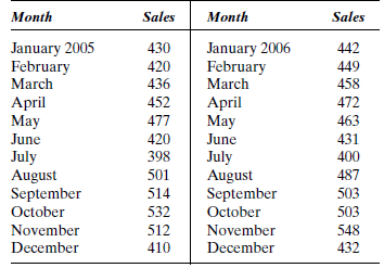
Apex Mutual Fund invests primarily in technology stocks. The price of the fund at the end of each month for the 12 months of 2006 is shown in Table P-6.
a. Find the forecast value of the mutual fund for each month by using a naive model (see Equation 4.1). The value for December 2005 was 19.00.
b. Evaluate this forecasting method using the MAD.
c. Evaluate this forecasting method using the MSE.
d. Evaluate this forecasting method using the MAPE.
e. Evaluate this forecasting method using the MPE.
f. Using a naive model, forecast the mutual fund price for January 2007.
g. Write a memo summarizing your findings.
TABLE P-6
Question
Question
Given the series Y t in Table P-8:
a. What is the forecast for period 9, using a five-period moving average?
b. If simple exponential smoothing with a smoothing constant of.4 is used, what is the forecast for time period 4?
c. In part b, what is the forecast error for time period 3?
TABLE P-8
a. What is the forecast for period 9, using a five-period moving average?
b. If simple exponential smoothing with a smoothing constant of.4 is used, what is the forecast for time period 4?
c. In part b, what is the forecast error for time period 3?
TABLE P-8
Question
The yield on a general obligation bond for the city of Davenport fluctuates with the market. The monthly quotations for 2006 are given in Table P-9.
TABLE P-9
a. Find the forecast value of the yield for the obligation bonds for each month, starting with April, using a three-month moving average.
b. Find the forecast value of the yield for the obligation bonds for each month, starting with June, using a five-month moving average.
c. Evaluate these forecasting methods using the MAD.
d. Evaluate these forecasting methods using the MSE.
e. Evaluate these forecasting methods using the MAPE.
f. Evaluate these forecasting methods using the MPE.
g. Forecast the yield for January 2007 using the better technique.
h. Write a memo summarizing your findings.
Question
Question
The Hughes Supply Company uses an inventory management method to determine the monthly demands for various products. The demand values for the last 12 months of each product have been recorded and are available for future forecasting. The demand values for the 12 months of 2006 for one electrical fixture are presented in Table P-11.
TABLE P-11
Source: Based on Hughes Supply Company records.
Use exponential smoothing with a smoothing constant of.5 and an initial value of 205 to forecast the demand for January 2007.
TABLE P-11
Source: Based on Hughes Supply Company records.
Use exponential smoothing with a smoothing constant of.5 and an initial value of 205 to forecast the demand for January 2007.
Question
General American Investors Company, a closed-end regulated investment management company, invests primarily in medium- and high-quality stocks. Jim Campbell is studying the asset value per share for this company and would like to forecast this variable for the remaining quarters of 1996. The data are presented in Table P-12.
Evaluate the ability to forecast the asset value per share variable of the following forecasting methods: naive, moving average, and exponential smoothing. When you compare techniques, take into consideration that the actual asset value per share for the second quarter of 1996 was 26.47. Write a report for Jim indicating which method he should use and why.
TABLE P-12 General American Investors Company Assets per Share, 1985-1996
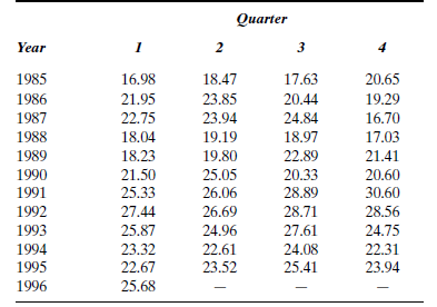
Source: The Value Line Investment Survey (New York: Value Line, 1990, 1993, 1996).
Evaluate the ability to forecast the asset value per share variable of the following forecasting methods: naive, moving average, and exponential smoothing. When you compare techniques, take into consideration that the actual asset value per share for the second quarter of 1996 was 26.47. Write a report for Jim indicating which method he should use and why.
TABLE P-12 General American Investors Company Assets per Share, 1985-1996
Source: The Value Line Investment Survey (New York: Value Line, 1990, 1993, 1996).
Question
Southdown, Inc., the nation's third largest cement producer, is pushing ahead with a waste fuel burning program. The cost for Southdown will total about $37 million. For this reason, it is extremely important for the company to have an accurate forecast of revenues for the first quarter of 2000. The data are presented in Table P-13.
a. Use exponential smoothing with a smoothing constant of.4 and an initial value of 77.4 to forecast the quarterly revenues for the first quarter of 2000.
b. Now use a smoothing constant of.6 and an initial value of 77.4 to forecast the quarterly revenues for the first quarter of 2000.
c. Which smoothing constant provides the better forecast?
d. Refer to part c. Examine the residual autocorrelations. Are you happy with simple exponential smoothing for this example? Explain.
TABLE P-13 Southdown Revenues, 1986-1999
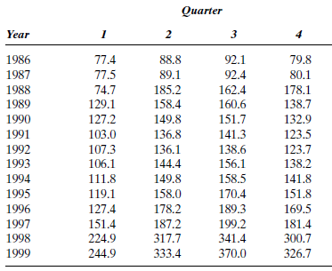
Source: The Value Line Investment Survey (New York: Value Line, 1990, 1993, 1996, 1999).
a. Use exponential smoothing with a smoothing constant of.4 and an initial value of 77.4 to forecast the quarterly revenues for the first quarter of 2000.
b. Now use a smoothing constant of.6 and an initial value of 77.4 to forecast the quarterly revenues for the first quarter of 2000.
c. Which smoothing constant provides the better forecast?
d. Refer to part c. Examine the residual autocorrelations. Are you happy with simple exponential smoothing for this example? Explain.
TABLE P-13 Southdown Revenues, 1986-1999
Source: The Value Line Investment Survey (New York: Value Line, 1990, 1993, 1996, 1999).
Question
The Triton Energy Corporation explores for and produces oil and gas. Company president Gail Freeman wants to have her company's analyst forecast the company's sales per share for 2000. This will be an important forecast, since Triton's restructuring plans have hit a snag. The data are presented in Table P-14.
Determine the best forecasting method and forecast sales per share for 2000.
TABLE P-14 Triton Sales per Share, 1974-1999
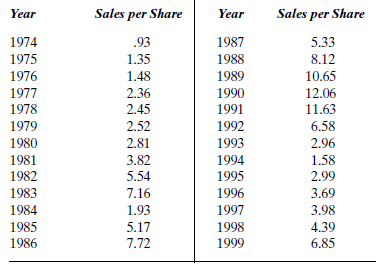
Source: The Value Line Investment Survey (New York: Value Line, 1990, 1993, 1996, 1999)
Determine the best forecasting method and forecast sales per share for 2000.
TABLE P-14 Triton Sales per Share, 1974-1999
Source: The Value Line Investment Survey (New York: Value Line, 1990, 1993, 1996, 1999)
Question
The Consolidated Edison Company sells electricity (82% of revenues), gas (13%), and steam (5%) in New York City and Westchester County. Bart Thomas, company forecaster, is assigned the task of forecasting the company's quarterly revenues for the rest of 2002 and all of 2003. He collects the data shown in Table P-15.
Determine the best forecasting technique and forecast quarterly revenue for the rest of 2002 and all of 2003.
TABLE P-15 Quarterly Revenues for Consolidated Edison ($ millions), 1985-June 2002
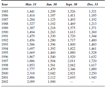
Source: The Value Line Investment Survey (New York: Value Line, 1990, 1993, 1996, 1999, 2001).
Determine the best forecasting technique and forecast quarterly revenue for the rest of 2002 and all of 2003.
TABLE P-15 Quarterly Revenues for Consolidated Edison ($ millions), 1985-June 2002
Source: The Value Line Investment Survey (New York: Value Line, 1990, 1993, 1996, 1999, 2001).
Question
A job-shop manufacturer that specializes in replacement parts has no forecasting system in place and manufactures products based on last month's sales. Twenty-four months of sales data are available and are given in Table P-16.
a. Plot the sales data as a time series. Are the data seasonal?
Hint: For monthly data, the seasonal period is s = 12. Is there a pattern (e.g., summer sales relatively low, fall sales relatively high) that tends to repeat itself every 12 months?
TABLE P-16
b. Use a naive model to generate monthly sales forecasts (e.g., the February 2005 forecast is given by the January 2005 value, and so forth). Compute the MAPE.
c. Use simple exponential smoothing with a smoothing constant of.5 and an initial smoothed value of 430 to generate sales forecasts for each month. Compute the MAPE.
d. Do you think either of the models in parts b and c is likely to generate accurate forecasts for future monthly sales? Explain.
e. Use Minitab and Winters' multiplicative smoothing method with smoothing constants ? = ? = ? =.5 to generate a forecast for January 2007. Save the residuals.
f. Refer to part e. Compare the MAPE for Winters' method from the computer printout with the MAPE s in parts b and c. Which of the three forecasting procedures do you prefer?
g. Refer to part e. Compute the autocorrelations (for six lags) for the residuals from Winters' multiplicative procedure. Do the residual autocorrelations suggest that Winters' procedure works well for these data? Explain.
Question
Question
Table P-18 contains the number of severe earthquakes (those with a Richter scale magnitude of 7 and above) per year for the years 1900-1999.
TABLE P-18 Number of Severe Earthquakes, 1900-1999
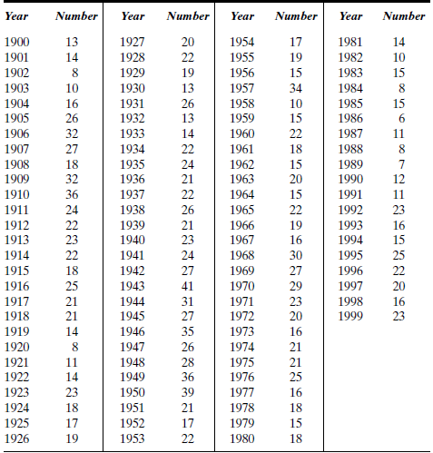
Source: U.S. Geological Survey Earthquake Hazard Program.
a. Use Minitab to smooth the earthquake data with moving averages of orders k = 5, 10, and 15. Describe the nature of the smoothing as the order of the moving average increases. Do you think there might be a cycle in these data? If so, provide an estimate of the length (in years) of the cycle.
b. Use Minitab to smooth the earthquake data using simple exponential smoothing. Store the residuals and generate a forecast for the number of severe earthquakes in the year 2000. Compute the residual autocorrelations. Does simple exponential smoothing provide a reasonable fit to these data? Explain.
c. Is there a seasonal component in the earthquake data? Why or why not?
TABLE P-18 Number of Severe Earthquakes, 1900-1999
Source: U.S. Geological Survey Earthquake Hazard Program.
a. Use Minitab to smooth the earthquake data with moving averages of orders k = 5, 10, and 15. Describe the nature of the smoothing as the order of the moving average increases. Do you think there might be a cycle in these data? If so, provide an estimate of the length (in years) of the cycle.
b. Use Minitab to smooth the earthquake data using simple exponential smoothing. Store the residuals and generate a forecast for the number of severe earthquakes in the year 2000. Compute the residual autocorrelations. Does simple exponential smoothing provide a reasonable fit to these data? Explain.
c. Is there a seasonal component in the earthquake data? Why or why not?
Question
Question
Table P-20 contains quarterly sales ($MM) of The Gap for fiscal years 1980-2004.
Plot The Gap sales data as a time series and examine its properties. The objective is to generate forecasts of sales for the four quarters of 2005. Select an appropriate smoothing method for forecasting and justify your choice.
TABLE P-20 Quarterly Sales for The Gap, Fiscal Years 1980-2004
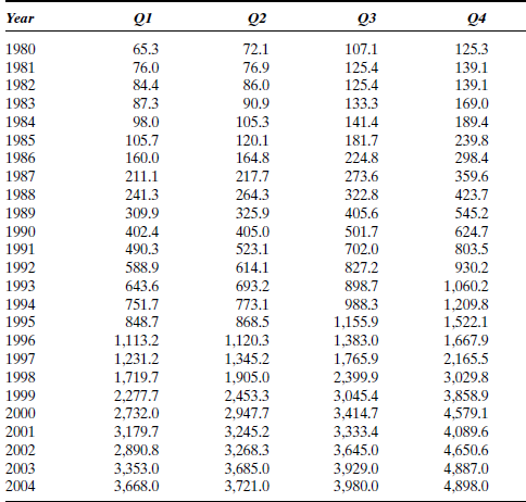
Source: Based on The Value Line Investment Survey (New York: Value Line, various years), and 10K filings with the Securities and Exchange Commission.
Plot The Gap sales data as a time series and examine its properties. The objective is to generate forecasts of sales for the four quarters of 2005. Select an appropriate smoothing method for forecasting and justify your choice.
TABLE P-20 Quarterly Sales for The Gap, Fiscal Years 1980-2004
Source: Based on The Value Line Investment Survey (New York: Value Line, various years), and 10K filings with the Securities and Exchange Commission.
Question
THE SOLAR ALTERNATIVE COMPANY
The Solar Alternative Company is about to enter its third year of operation. Bob and Mary Johnson, who both teach science in the local high school, founded the company. The Johnsons started the Solar Alternative Company to supplement their teaching income. Based on their research into solar energy systems, they were able to put together a solar system for heating domestic hot water. The system consists of a 100-gallon fiberglass storage tank, two 36-foot solar panels, electronic controls, PVC pipe, and miscellaneous fittings.
The payback period on the system is 10 years. Although this situation does not present an attractive investment opportunity from a financial point of view, there is sufficient interest in the novelty of the concept to provide a moderate level of sales. The Johnsons clear about $75 on the $2,000 price of an installed system, after costs and expenses. Material and equipment costs account for 75% of the installed system cost. An advantage that helps to offset the low profit margin is the fact that the product is not profitable enough to generate any significant competition from heating contractors. The Johnsons operate the business out of their home. They have an office in the basement, and their one-car garage is used exclusively to store the system components and materials. As a result, overhead is at a minimum. The Johnsons enjoy a modest supplemental income from the company's operation. The business also provides a number of tax advantages.
Bob and Mary are pleased with the growth of the business. Although sales vary from month to month, overall the second year was much better than the first. Many of the second-year customers are neighbors of people who had purchased the system in the first year. Apparently, after seeing the system operate successfully for a year, others were willing to try the solar concept. Sales occur throughout the year. Demand for the system is greatest in late summer and early fall, when homeowners typically make plans to winterize their homes for the upcoming heating season.
With the anticipated growth in the business, the Johnsons felt that they needed a sales forecast to manage effectively in the coming year. It usually takes 60 to 90 days to receive storage tanks after placing the order. The solar panels are available off the shelf most of the year. However, in the late summer and throughout the fall, the lead time can be as much as 90 to 100 days. Although there is limited competition, lost sales are nevertheless a real possibility if the potential customer is asked to wait several months for installation. Perhaps more important is the need to make accurate sales projections to take advantage of quantity discount buying. These factors, when combined with the high cost of system components and the limited storage space available in the garage, make it necessary to develop a reliable forecast. The sales history for the company's first two years is given in Table 4-10.
TABLE 4-10

Identify the model Bob and Mary should use as the basis for their business planning in 2007, and discuss why you selected this model.
The Solar Alternative Company is about to enter its third year of operation. Bob and Mary Johnson, who both teach science in the local high school, founded the company. The Johnsons started the Solar Alternative Company to supplement their teaching income. Based on their research into solar energy systems, they were able to put together a solar system for heating domestic hot water. The system consists of a 100-gallon fiberglass storage tank, two 36-foot solar panels, electronic controls, PVC pipe, and miscellaneous fittings.
The payback period on the system is 10 years. Although this situation does not present an attractive investment opportunity from a financial point of view, there is sufficient interest in the novelty of the concept to provide a moderate level of sales. The Johnsons clear about $75 on the $2,000 price of an installed system, after costs and expenses. Material and equipment costs account for 75% of the installed system cost. An advantage that helps to offset the low profit margin is the fact that the product is not profitable enough to generate any significant competition from heating contractors. The Johnsons operate the business out of their home. They have an office in the basement, and their one-car garage is used exclusively to store the system components and materials. As a result, overhead is at a minimum. The Johnsons enjoy a modest supplemental income from the company's operation. The business also provides a number of tax advantages.
Bob and Mary are pleased with the growth of the business. Although sales vary from month to month, overall the second year was much better than the first. Many of the second-year customers are neighbors of people who had purchased the system in the first year. Apparently, after seeing the system operate successfully for a year, others were willing to try the solar concept. Sales occur throughout the year. Demand for the system is greatest in late summer and early fall, when homeowners typically make plans to winterize their homes for the upcoming heating season.
With the anticipated growth in the business, the Johnsons felt that they needed a sales forecast to manage effectively in the coming year. It usually takes 60 to 90 days to receive storage tanks after placing the order. The solar panels are available off the shelf most of the year. However, in the late summer and throughout the fall, the lead time can be as much as 90 to 100 days. Although there is limited competition, lost sales are nevertheless a real possibility if the potential customer is asked to wait several months for installation. Perhaps more important is the need to make accurate sales projections to take advantage of quantity discount buying. These factors, when combined with the high cost of system components and the limited storage space available in the garage, make it necessary to develop a reliable forecast. The sales history for the company's first two years is given in Table 4-10.
TABLE 4-10
Identify the model Bob and Mary should use as the basis for their business planning in 2007, and discuss why you selected this model.
Question
THE SOLAR ALTERNATIVE COMPANY
The Solar Alternative Company is about to enter its third year of operation. Bob and Mary Johnson, who both teach science in the local high school, founded the company. The Johnsons started the Solar Alternative Company to supplement their teaching income. Based on their research into solar energy systems, they were able to put together a solar system for heating domestic hot water. The system consists of a 100-gallon fiberglass storage tank, two 36-foot solar panels, electronic controls, PVC pipe, and miscellaneous fittings.
The payback period on the system is 10 years. Although this situation does not present an attractive investment opportunity from a financial point of view, there is sufficient interest in the novelty of the concept to provide a moderate level of sales. The Johnsons clear about $75 on the $2,000 price of an installed system, after costs and expenses. Material and equipment costs account for 75% of the installed system cost. An advantage that helps to offset the low profit margin is the fact that the product is not profitable enough to generate any significant competition from heating contractors. The Johnsons operate the business out of their home. They have an office in the basement, and their one-car garage is used exclusively to store the system components and materials. As a result, overhead is at a minimum. The Johnsons enjoy a modest supplemental income from the company's operation. The business also provides a number of tax advantages.
Bob and Mary are pleased with the growth of the business. Although sales vary from month to month, overall the second year was much better than the first. Many of the second-year customers are neighbors of people who had purchased the system in the first year. Apparently, after seeing the system operate successfully for a year, others were willing to try the solar concept. Sales occur throughout the year. Demand for the system is greatest in late summer and early fall, when homeowners typically make plans to winterize their homes for the upcoming heating season.
With the anticipated growth in the business, the Johnsons felt that they needed a sales forecast to manage effectively in the coming year. It usually takes 60 to 90 days to receive storage tanks after placing the order. The solar panels are available off the shelf most of the year. However, in the late summer and throughout the fall, the lead time can be as much as 90 to 100 days. Although there is limited competition, lost sales are nevertheless a real possibility if the potential customer is asked to wait several months for installation. Perhaps more important is the need to make accurate sales projections to take advantage of quantity discount buying. These factors, when combined with the high cost of system components and the limited storage space available in the garage, make it necessary to develop a reliable forecast. The sales history for the company's first two years is given in Table 4-10.
TABLE 4-10
Forecast sales for 2007.
Question
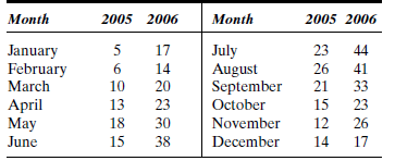
TUX
John Mosby, owner of several Mr. Tux rental stores, is beginning to forecast his most important business variable, monthly dollar sales (see the Mr. Tux cases in previous chapters). One of his employees, Virginia Perot, gathered the sales data shown in Case 2-2. John now wants to create a forecast based on these sales data using moving average and exponential smoothing techniques.
John used Minitab in Case 3-2 to determine that these data are both trending and seasonal. He has been told that simple moving averages and exponential smoothing techniques will not work with these data but decides to find out for himself.
He begins by trying a three-month moving average. The program calculates several summary forecast error measurements. These values summarize the errors found in predicting actual historical data values using a three-month moving average. John decides to record two of these error measurements:
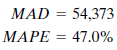
The MAD (mean absolute deviation) is the average absolute error made in forecasting past values. Each forecast using the three-month moving average method is off by an average of 54,373. The MAPE (mean absolute percentage error) shows the error as a percentage of the actual value to be forecast. The average error using the three-month moving average technique is 47%, or almost half as large as the value to be forecast.
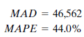
Next, John tries simple exponential smoothing. The program asks him to input the smoothing constant ( ? ) to be used or to ask that the optimum ? value be calculated. John does the latter, and the program finds the optimum ? value to be.867. Again he records the appropriate error measurements:
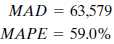
John asks the program to use Holt's linear exponential smoothing on his data. This program uses the exponential smoothing method but can account for a trend in the data as well. John has the program use a smoothing constant of.4 for both ? and ?. The two summary error measurements for Holt's method are

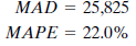
John is surprised to find larger measurement errors for this technique. He decides that the seasonal aspect of the data is the problem. Winters' multiplicative exponential smoothing is the next method John tries. This method can account for seasonal factors as well as trend. John uses smoothing constants of ? =.2, ? =.2, and ? =.2. Error measurements are

When John sits down and begins studying the results of his analysis, he is disappointed. The Winters' method is a big improvement; however, the MAPE is still 22%. He had hoped that one of the methods he used would result in accurate forecasts of past periods; he could then use this method to forecast the sales levels for coming months over the next year. But the average absolute errors (MADs) and percentage errors ( MAPE s) for these methods lead him to look for another way of forecasting.
Summarize the forecast error level for the best method John has found using Minitab.
John Mosby, owner of several Mr. Tux rental stores, is beginning to forecast his most important business variable, monthly dollar sales (see the Mr. Tux cases in previous chapters). One of his employees, Virginia Perot, gathered the sales data shown in Case 2-2. John now wants to create a forecast based on these sales data using moving average and exponential smoothing techniques.
John used Minitab in Case 3-2 to determine that these data are both trending and seasonal. He has been told that simple moving averages and exponential smoothing techniques will not work with these data but decides to find out for himself.
He begins by trying a three-month moving average. The program calculates several summary forecast error measurements. These values summarize the errors found in predicting actual historical data values using a three-month moving average. John decides to record two of these error measurements:
The MAD (mean absolute deviation) is the average absolute error made in forecasting past values. Each forecast using the three-month moving average method is off by an average of 54,373. The MAPE (mean absolute percentage error) shows the error as a percentage of the actual value to be forecast. The average error using the three-month moving average technique is 47%, or almost half as large as the value to be forecast.
Next, John tries simple exponential smoothing. The program asks him to input the smoothing constant ( ? ) to be used or to ask that the optimum ? value be calculated. John does the latter, and the program finds the optimum ? value to be.867. Again he records the appropriate error measurements:
John asks the program to use Holt's linear exponential smoothing on his data. This program uses the exponential smoothing method but can account for a trend in the data as well. John has the program use a smoothing constant of.4 for both ? and ?. The two summary error measurements for Holt's method are
John is surprised to find larger measurement errors for this technique. He decides that the seasonal aspect of the data is the problem. Winters' multiplicative exponential smoothing is the next method John tries. This method can account for seasonal factors as well as trend. John uses smoothing constants of ? =.2, ? =.2, and ? =.2. Error measurements are
When John sits down and begins studying the results of his analysis, he is disappointed. The Winters' method is a big improvement; however, the MAPE is still 22%. He had hoped that one of the methods he used would result in accurate forecasts of past periods; he could then use this method to forecast the sales levels for coming months over the next year. But the average absolute errors (MADs) and percentage errors ( MAPE s) for these methods lead him to look for another way of forecasting.
Summarize the forecast error level for the best method John has found using Minitab.
Question
TUX
John Mosby, owner of several Mr. Tux rental stores, is beginning to forecast his most important business variable, monthly dollar sales (see the Mr. Tux cases in previous chapters). One of his employees, Virginia Perot, gathered the sales data shown in Case 2-2. John now wants to create a forecast based on these sales data using moving average and exponential smoothing techniques.
John used Minitab in Case 3-2 to determine that these data are both trending and seasonal. He has been told that simple moving averages and exponential smoothing techniques will not work with these data but decides to find out for himself.
He begins by trying a three-month moving average. The program calculates several summary forecast error measurements. These values summarize the errors found in predicting actual historical data values using a three-month moving average. John decides to record two of these error measurements:

The MAD (mean absolute deviation) is the average absolute error made in forecasting past values. Each forecast using the three-month moving average method is off by an average of 54,373. The MAPE (mean absolute percentage error) shows the error as a percentage of the actual value to be forecast. The average error using the three-month moving average technique is 47%, or almost half as large as the value to be forecast.
Next, John tries simple exponential smoothing. The program asks him to input the smoothing constant ( ? ) to be used or to ask that the optimum ? value be calculated. John does the latter, and the program finds the optimum ? value to be.867. Again he records the appropriate error measurements:

John asks the program to use Holt's linear exponential smoothing on his data. This program uses the exponential smoothing method but can account for a trend in the data as well. John has the program use a smoothing constant of.4 for both ? and ?. The two summary error measurements for Holt's method are
John is surprised to find larger measurement errors for this technique. He decides that the seasonal aspect of the data is the problem. Winters' multiplicative exponential smoothing is the next method John tries. This method can account for seasonal factors as well as trend. John uses smoothing constants of ? =.2, ? =.2, and ? =.2. Error measurements are

When John sits down and begins studying the results of his analysis, he is disappointed. The Winters' method is a big improvement; however, the MAPE is still 22%. He had hoped that one of the methods he used would result in accurate forecasts of past periods; he could then use this method to forecast the sales levels for coming months over the next year. But the average absolute errors (MADs) and percentage errors ( MAPE s) for these methods lead him to look for another way of forecasting.
John used the Minitab default values for ? , ? , and ?. John thinks there are other choices for these parameters that would lead to smaller error measurements. Do you agree?
John Mosby, owner of several Mr. Tux rental stores, is beginning to forecast his most important business variable, monthly dollar sales (see the Mr. Tux cases in previous chapters). One of his employees, Virginia Perot, gathered the sales data shown in Case 2-2. John now wants to create a forecast based on these sales data using moving average and exponential smoothing techniques.
John used Minitab in Case 3-2 to determine that these data are both trending and seasonal. He has been told that simple moving averages and exponential smoothing techniques will not work with these data but decides to find out for himself.
He begins by trying a three-month moving average. The program calculates several summary forecast error measurements. These values summarize the errors found in predicting actual historical data values using a three-month moving average. John decides to record two of these error measurements:
The MAD (mean absolute deviation) is the average absolute error made in forecasting past values. Each forecast using the three-month moving average method is off by an average of 54,373. The MAPE (mean absolute percentage error) shows the error as a percentage of the actual value to be forecast. The average error using the three-month moving average technique is 47%, or almost half as large as the value to be forecast.
Next, John tries simple exponential smoothing. The program asks him to input the smoothing constant ( ? ) to be used or to ask that the optimum ? value be calculated. John does the latter, and the program finds the optimum ? value to be.867. Again he records the appropriate error measurements:
John asks the program to use Holt's linear exponential smoothing on his data. This program uses the exponential smoothing method but can account for a trend in the data as well. John has the program use a smoothing constant of.4 for both ? and ?. The two summary error measurements for Holt's method are
John is surprised to find larger measurement errors for this technique. He decides that the seasonal aspect of the data is the problem. Winters' multiplicative exponential smoothing is the next method John tries. This method can account for seasonal factors as well as trend. John uses smoothing constants of ? =.2, ? =.2, and ? =.2. Error measurements are
When John sits down and begins studying the results of his analysis, he is disappointed. The Winters' method is a big improvement; however, the MAPE is still 22%. He had hoped that one of the methods he used would result in accurate forecasts of past periods; he could then use this method to forecast the sales levels for coming months over the next year. But the average absolute errors (MADs) and percentage errors ( MAPE s) for these methods lead him to look for another way of forecasting.
John used the Minitab default values for ? , ? , and ?. John thinks there are other choices for these parameters that would lead to smaller error measurements. Do you agree?
Question
TUX
John Mosby, owner of several Mr. Tux rental stores, is beginning to forecast his most important business variable, monthly dollar sales (see the Mr. Tux cases in previous chapters). One of his employees, Virginia Perot, gathered the sales data shown in Case 2-2. John now wants to create a forecast based on these sales data using moving average and exponential smoothing techniques.
John used Minitab in Case 3-2 to determine that these data are both trending and seasonal. He has been told that simple moving averages and exponential smoothing techniques will not work with these data but decides to find out for himself.
He begins by trying a three-month moving average. The program calculates several summary forecast error measurements. These values summarize the errors found in predicting actual historical data values using a three-month moving average. John decides to record two of these error measurements:

The MAD (mean absolute deviation) is the average absolute error made in forecasting past values. Each forecast using the three-month moving average method is off by an average of 54,373. The MAPE (mean absolute percentage error) shows the error as a percentage of the actual value to be forecast. The average error using the three-month moving average technique is 47%, or almost half as large as the value to be forecast.
Next, John tries simple exponential smoothing. The program asks him to input the smoothing constant ( ? ) to be used or to ask that the optimum ? value be calculated. John does the latter, and the program finds the optimum ? value to be.867. Again he records the appropriate error measurements:

John asks the program to use Holt's linear exponential smoothing on his data. This program uses the exponential smoothing method but can account for a trend in the data as well. John has the program use a smoothing constant of.4 for both ? and ?. The two summary error measurements for Holt's method are

John is surprised to find larger measurement errors for this technique. He decides that the seasonal aspect of the data is the problem. Winters' multiplicative exponential smoothing is the next method John tries. This method can account for seasonal factors as well as trend. John uses smoothing constants of ? =.2, ? =.2, and ? =.2. Error measurements are
When John sits down and begins studying the results of his analysis, he is disappointed. The Winters' method is a big improvement; however, the MAPE is still 22%. He had hoped that one of the methods he used would result in accurate forecasts of past periods; he could then use this method to forecast the sales levels for coming months over the next year. But the average absolute errors (MADs) and percentage errors ( MAPE s) for these methods lead him to look for another way of forecasting.
Although disappointed with his initial results, this may be the best he can do with smoothing methods. What should John do, for example, to determine the adequacy of the Winters' forecasting technique?
John Mosby, owner of several Mr. Tux rental stores, is beginning to forecast his most important business variable, monthly dollar sales (see the Mr. Tux cases in previous chapters). One of his employees, Virginia Perot, gathered the sales data shown in Case 2-2. John now wants to create a forecast based on these sales data using moving average and exponential smoothing techniques.
John used Minitab in Case 3-2 to determine that these data are both trending and seasonal. He has been told that simple moving averages and exponential smoothing techniques will not work with these data but decides to find out for himself.
He begins by trying a three-month moving average. The program calculates several summary forecast error measurements. These values summarize the errors found in predicting actual historical data values using a three-month moving average. John decides to record two of these error measurements:
The MAD (mean absolute deviation) is the average absolute error made in forecasting past values. Each forecast using the three-month moving average method is off by an average of 54,373. The MAPE (mean absolute percentage error) shows the error as a percentage of the actual value to be forecast. The average error using the three-month moving average technique is 47%, or almost half as large as the value to be forecast.
Next, John tries simple exponential smoothing. The program asks him to input the smoothing constant ( ? ) to be used or to ask that the optimum ? value be calculated. John does the latter, and the program finds the optimum ? value to be.867. Again he records the appropriate error measurements:
John asks the program to use Holt's linear exponential smoothing on his data. This program uses the exponential smoothing method but can account for a trend in the data as well. John has the program use a smoothing constant of.4 for both ? and ?. The two summary error measurements for Holt's method are
John is surprised to find larger measurement errors for this technique. He decides that the seasonal aspect of the data is the problem. Winters' multiplicative exponential smoothing is the next method John tries. This method can account for seasonal factors as well as trend. John uses smoothing constants of ? =.2, ? =.2, and ? =.2. Error measurements are
When John sits down and begins studying the results of his analysis, he is disappointed. The Winters' method is a big improvement; however, the MAPE is still 22%. He had hoped that one of the methods he used would result in accurate forecasts of past periods; he could then use this method to forecast the sales levels for coming months over the next year. But the average absolute errors (MADs) and percentage errors ( MAPE s) for these methods lead him to look for another way of forecasting.
Although disappointed with his initial results, this may be the best he can do with smoothing methods. What should John do, for example, to determine the adequacy of the Winters' forecasting technique?
Question
TUX
John Mosby, owner of several Mr. Tux rental stores, is beginning to forecast his most important business variable, monthly dollar sales (see the Mr. Tux cases in previous chapters). One of his employees, Virginia Perot, gathered the sales data shown in Case 2-2. John now wants to create a forecast based on these sales data using moving average and exponential smoothing techniques.
John used Minitab in Case 3-2 to determine that these data are both trending and seasonal. He has been told that simple moving averages and exponential smoothing techniques will not work with these data but decides to find out for himself.
He begins by trying a three-month moving average. The program calculates several summary forecast error measurements. These values summarize the errors found in predicting actual historical data values using a three-month moving average. John decides to record two of these error measurements:

The MAD (mean absolute deviation) is the average absolute error made in forecasting past values. Each forecast using the three-month moving average method is off by an average of 54,373. The MAPE (mean absolute percentage error) shows the error as a percentage of the actual value to be forecast. The average error using the three-month moving average technique is 47%, or almost half as large as the value to be forecast.
Next, John tries simple exponential smoothing. The program asks him to input the smoothing constant ( ? ) to be used or to ask that the optimum ? value be calculated. John does the latter, and the program finds the optimum ? value to be.867. Again he records the appropriate error measurements:

John asks the program to use Holt's linear exponential smoothing on his data. This program uses the exponential smoothing method but can account for a trend in the data as well. John has the program use a smoothing constant of.4 for both ? and ?. The two summary error measurements for Holt's method are

John is surprised to find larger measurement errors for this technique. He decides that the seasonal aspect of the data is the problem. Winters' multiplicative exponential smoothing is the next method John tries. This method can account for seasonal factors as well as trend. John uses smoothing constants of ? =.2, ? =.2, and ? =.2. Error measurements are

When John sits down and begins studying the results of his analysis, he is disappointed. The Winters' method is a big improvement; however, the MAPE is still 22%. He had hoped that one of the methods he used would result in accurate forecasts of past periods; he could then use this method to forecast the sales levels for coming months over the next year. But the average absolute errors (MADs) and percentage errors ( MAPE s) for these methods lead him to look for another way of forecasting.
Although not calculated directly in Minitab, the MPE (mean percentage error) measures forecast bias. What is the ideal value for the MPE ? What is the implication of a negative sign on the MPE ?
John Mosby, owner of several Mr. Tux rental stores, is beginning to forecast his most important business variable, monthly dollar sales (see the Mr. Tux cases in previous chapters). One of his employees, Virginia Perot, gathered the sales data shown in Case 2-2. John now wants to create a forecast based on these sales data using moving average and exponential smoothing techniques.
John used Minitab in Case 3-2 to determine that these data are both trending and seasonal. He has been told that simple moving averages and exponential smoothing techniques will not work with these data but decides to find out for himself.
He begins by trying a three-month moving average. The program calculates several summary forecast error measurements. These values summarize the errors found in predicting actual historical data values using a three-month moving average. John decides to record two of these error measurements:
The MAD (mean absolute deviation) is the average absolute error made in forecasting past values. Each forecast using the three-month moving average method is off by an average of 54,373. The MAPE (mean absolute percentage error) shows the error as a percentage of the actual value to be forecast. The average error using the three-month moving average technique is 47%, or almost half as large as the value to be forecast.
Next, John tries simple exponential smoothing. The program asks him to input the smoothing constant ( ? ) to be used or to ask that the optimum ? value be calculated. John does the latter, and the program finds the optimum ? value to be.867. Again he records the appropriate error measurements:
John asks the program to use Holt's linear exponential smoothing on his data. This program uses the exponential smoothing method but can account for a trend in the data as well. John has the program use a smoothing constant of.4 for both ? and ?. The two summary error measurements for Holt's method are
John is surprised to find larger measurement errors for this technique. He decides that the seasonal aspect of the data is the problem. Winters' multiplicative exponential smoothing is the next method John tries. This method can account for seasonal factors as well as trend. John uses smoothing constants of ? =.2, ? =.2, and ? =.2. Error measurements are
When John sits down and begins studying the results of his analysis, he is disappointed. The Winters' method is a big improvement; however, the MAPE is still 22%. He had hoped that one of the methods he used would result in accurate forecasts of past periods; he could then use this method to forecast the sales levels for coming months over the next year. But the average absolute errors (MADs) and percentage errors ( MAPE s) for these methods lead him to look for another way of forecasting.
Although not calculated directly in Minitab, the MPE (mean percentage error) measures forecast bias. What is the ideal value for the MPE ? What is the implication of a negative sign on the MPE ?
Question
Question
Question
Question
Question
Question
Question
Question
Question
Question
FIVE-YEAR REVENUE PROJECTION FOR DOWNTOWN RADIOLOGY
Some years ago Downtown Radiology developed a medical imaging center that was more complete and technologically advanced than any located in an area of eastern Washington and northern Idaho called the Inland Empire. The equipment planned for the center equaled or surpassed the imaging facilities of all medical centers in the region. The center initially contained a 9800 series CT scanner and nuclear magnetic resonance imaging (MRI) equipment. The center also included ultrasound, nuclear medicine, digital subtraction angiography (DSA), mammography, and conventional radiology and fluoroscopy equipment. Ownership interest was made available in a type of public offering, and Downtown Radiology used an independent evaluation of the market. Professional Marketing Associates, Inc., evaluated the market and completed a five-year projection of revenue.
STATEMENT OF THE PROBLEM
The purpose of this study is to forecast revenue for the next five years for the proposed medical imaging center, assuming you are employed by Professional Marketing Associates, Inc., in the year 1984.
OBJECTIVES
The objectives of this study are to
• Identify market areas for each type of medical procedure to be offered by the new facility.
• Gather and analyze existing data on market area revenue for each type of procedure to be offered by the new facility.
• Identify trends in the health care industry that will positively or negatively affect revenue of procedures to be provided by the proposed facility.
• Identify factors in the business, marketing, or facility planning of the new venture that will positively or negatively impact revenue projections.
• Analyze past procedures of Downtown Radiology when compiling a database for the forecasting model to be developed.
• Utilize the appropriate quantitative forecasting model to arrive at five-year revenue projections for the proposed center.
METHODOLOGY
Medical Procedures
The following steps were implemented in order to complete the five-year projection of revenue. An analysis of the past number of procedures was performed. The appropriate forecasting model was developed and used to determine a starting point for the projection of each procedure.
1. The market area was determined for each type of procedure, and population forecasts were obtained for 1986 and 1990.
2. Doctor referral patterns were studied to determine the percentage of doctors who refer to Downtown Radiology and the average number of referrals per doctor.
3. National rates were acquired from the National Center for Health Statistics. These rates were compared with actual numbers obtained from the Hospital Commission.
4. Downtown Radiology's market share was calculated based on actual CT scans in the market area. (Market share for other procedures was determined based on Downtown Radiology's share compared to rates provided by the National Center for Health Statistics.)
Assumptions
The following assumptions, which were necessary to develop a quantitative forecast, were made:
• The new imaging center will be operational, with all equipment functional except the MRI, on January 1, 1985.
• The nuclear magnetic resonance imaging equipment will be functional in April 1985.
• The offering of the limited partnership will be successfully marketed to at least 50 physicians in the service area.
• Physicians who have a financial interest in the new imaging center will increase their referrals to the center.
• There will be no other MRIs in the market area before 1987.
• The new imaging center will offer services at lower prices than the competition.
• An effective marketing effort will take place, especially concentrating on large employers, insurance groups, and unions.
• The MRI will replace approximately 60% of the head scans that are presently done with the CT scanner during the first six months of operation and 70% during the next 12 months.
• The general public will continue to pressure the health care industry to hold down costs.
• Costs of outlays in the health care industry rose 13.2% annually from 1971 to 1981. The Health Care Financing Administration estimates that the average annual rate of increase will be reduced to approximately 11% to 12% between 1981 and 1990 ( Industry Surveys, April 1984).
• Insurance firms will reimburse patients for (at worst) 0% up to (at best) 100% of the cost of magnetic resonance imaging ( Imaging News, February 1984).
Models
A forecast was developed for each procedure, based on past experience, industry rates, and reasonable assumptions. The models were developed based on the preceding assumptions; however, if the assumptions are not valid, the models will not be accurate.
ANALYSIS OF PAST DATA
Office X-Rays
The number of X-ray procedures performed was analyzed from July 1981 to May 1984. The data included diagnostic X-rays, gastrointestinal X-rays, breast imaging, injections, and special procedures. Examination of these data indicated that no trend or seasonal or cyclical pattern is present. For this reason, simple exponential smoothing was chosen as the appropriate forecasting method. Various smoothing constants were examined, and a smoothing constant of.3 was found to provide the best model. The results are presented in Figure 4-14. The forecast for period 36, June 1984, is 855 X-ray procedures.
Office Ultrasound
The number of ultrasound procedures performed was analyzed from July 1981 to May 1984. Figure 4-15 shows the data pattern. Again, no trend or seasonal or cyclical pattern was present. Exponential smoothing with a smoothing constant of ? =.5 was determined to provide the best model. The forecast for June 1984 plotted in Figure 4-15 is 127 ultrasound procedures.
The number of ultrasound procedures performed by the two mobile units owned by Downtown Radiology was analyzed from July 1981 to May 1984. Figure 4-16 shows the data pattern. An increasing trend is apparent and can be modeled using Holt's two-parameter linear exponential smoothing. Smoothing constants of ? =.5 and ? =.1 are used, and the forecast for period 36, June 1984, is 227.
FIGURE 4-14 Simple Exponential Smoothing: Downtown Radiology X-Rays
![FIVE-YEAR REVENUE PROJECTION FOR DOWNTOWN RADIOLOGY Some years ago Downtown Radiology developed a medical imaging center that was more complete and technologically advanced than any located in an area of eastern Washington and northern Idaho called the Inland Empire. The equipment planned for the center equaled or surpassed the imaging facilities of all medical centers in the region. The center initially contained a 9800 series CT scanner and nuclear magnetic resonance imaging (MRI) equipment. The center also included ultrasound, nuclear medicine, digital subtraction angiography (DSA), mammography, and conventional radiology and fluoroscopy equipment. Ownership interest was made available in a type of public offering, and Downtown Radiology used an independent evaluation of the market. Professional Marketing Associates, Inc., evaluated the market and completed a five-year projection of revenue. STATEMENT OF THE PROBLEM The purpose of this study is to forecast revenue for the next five years for the proposed medical imaging center, assuming you are employed by Professional Marketing Associates, Inc., in the year 1984. OBJECTIVES The objectives of this study are to • Identify market areas for each type of medical procedure to be offered by the new facility. • Gather and analyze existing data on market area revenue for each type of procedure to be offered by the new facility. • Identify trends in the health care industry that will positively or negatively affect revenue of procedures to be provided by the proposed facility. • Identify factors in the business, marketing, or facility planning of the new venture that will positively or negatively impact revenue projections. • Analyze past procedures of Downtown Radiology when compiling a database for the forecasting model to be developed. • Utilize the appropriate quantitative forecasting model to arrive at five-year revenue projections for the proposed center. METHODOLOGY Medical Procedures The following steps were implemented in order to complete the five-year projection of revenue. An analysis of the past number of procedures was performed. The appropriate forecasting model was developed and used to determine a starting point for the projection of each procedure. 1. The market area was determined for each type of procedure, and population forecasts were obtained for 1986 and 1990. 2. Doctor referral patterns were studied to determine the percentage of doctors who refer to Downtown Radiology and the average number of referrals per doctor. 3. National rates were acquired from the National Center for Health Statistics. These rates were compared with actual numbers obtained from the Hospital Commission. 4. Downtown Radiology's market share was calculated based on actual CT scans in the market area. (Market share for other procedures was determined based on Downtown Radiology's share compared to rates provided by the National Center for Health Statistics.) Assumptions The following assumptions, which were necessary to develop a quantitative forecast, were made: • The new imaging center will be operational, with all equipment functional except the MRI, on January 1, 1985. • The nuclear magnetic resonance imaging equipment will be functional in April 1985. • The offering of the limited partnership will be successfully marketed to at least 50 physicians in the service area. • Physicians who have a financial interest in the new imaging center will increase their referrals to the center. • There will be no other MRIs in the market area before 1987. • The new imaging center will offer services at lower prices than the competition. • An effective marketing effort will take place, especially concentrating on large employers, insurance groups, and unions. • The MRI will replace approximately 60% of the head scans that are presently done with the CT scanner during the first six months of operation and 70% during the next 12 months. • The general public will continue to pressure the health care industry to hold down costs. • Costs of outlays in the health care industry rose 13.2% annually from 1971 to 1981. The Health Care Financing Administration estimates that the average annual rate of increase will be reduced to approximately 11% to 12% between 1981 and 1990 ( Industry Surveys, April 1984). • Insurance firms will reimburse patients for (at worst) 0% up to (at best) 100% of the cost of magnetic resonance imaging ( Imaging News, February 1984). Models A forecast was developed for each procedure, based on past experience, industry rates, and reasonable assumptions. The models were developed based on the preceding assumptions; however, if the assumptions are not valid, the models will not be accurate. ANALYSIS OF PAST DATA Office X-Rays The number of X-ray procedures performed was analyzed from July 1981 to May 1984. The data included diagnostic X-rays, gastrointestinal X-rays, breast imaging, injections, and special procedures. Examination of these data indicated that no trend or seasonal or cyclical pattern is present. For this reason, simple exponential smoothing was chosen as the appropriate forecasting method. Various smoothing constants were examined, and a smoothing constant of.3 was found to provide the best model. The results are presented in Figure 4-14. The forecast for period 36, June 1984, is 855 X-ray procedures. Office Ultrasound The number of ultrasound procedures performed was analyzed from July 1981 to May 1984. Figure 4-15 shows the data pattern. Again, no trend or seasonal or cyclical pattern was present. Exponential smoothing with a smoothing constant of ? =.5 was determined to provide the best model. The forecast for June 1984 plotted in Figure 4-15 is 127 ultrasound procedures. The number of ultrasound procedures performed by the two mobile units owned by Downtown Radiology was analyzed from July 1981 to May 1984. Figure 4-16 shows the data pattern. An increasing trend is apparent and can be modeled using Holt's two-parameter linear exponential smoothing. Smoothing constants of ? =.5 and ? =.1 are used, and the forecast for period 36, June 1984, is 227. FIGURE 4-14 Simple Exponential Smoothing: Downtown Radiology X-Rays FIGURE 4-15 Simple Exponential Smoothing: Downtown Radiology Ultrasound FIGURE 4-16 Holt's Linear Exponential Smoothing: Downtown Radiology Nonoffice Ultrasound Nuclear Medicine Procedures The number of nuclear medicine procedures performed by the two mobile units owned by Downtown Radiology was analyzed from August 1982 to May 1984. Figure 4-17 shows the data pattern. The data were not seasonal and had no trend or cyclical pattern. For this reason, simple exponential smoothing was chosen as the appropriate forecasting method. A smoothing factor of ? =.5 was found to provide the best model. The forecast for period 23, June 1984, is 48 nuclear medicine procedures. FIGURE 4-17 Simple Exponential Smoothing: Downtown Radiology Nonoffice Nuclear Medicine Office CT Scans The number of CT scans performed was also analyzed from July 1981 to May 1984. Seasonality was not found, and the number of CT scans did not seem to have a trend. However, a cyclical pattern seemed to be present. Knowing how many scans were performed last month would be important in forecasting what is going to happen this month. An autoregressive model (see Chapters 8 and 9) was examined and compared to an exponential smoothing model with a smoothing constant of ? =.461. The larger smoothing constant gives the most recent observation more weight in the forecast. The exponential smoothing model was determined to be better than the autoregressive model, and Figure 4-18 shows the projection of the number of CT scans for period 36, June 1984, to be 221. FIGURE 4-18 Simple Exponential Smoothing: Downtown Radiology CT Scans MARKET AREA ANALYSIS Market areas were determined for procedures currently done by Downtown Radiology by examining patient records and doctor referral patterns. Market areas were determined for procedures not currently done by Downtown Radiology by investigating the competition and analyzing the geographical areas they served. CT Scanner Market Area The market area for CT scanning for the proposed medical imaging center includes Spokane, Whitman, Adams, Lincoln, Stevens, and Pend Oreille Counties in Washington and Bonner, Boundary, Kootenai, Benewah, and Shoshone Counties in Idaho. Based on the appropriate percentage projections, the CT scanning market area will have a population of 630,655 in 1985 and 696,018 in 1990. Quantitative Estimates To project revenue, it is necessary to determine certain quantitative estimates. The most important estimate involves the number of doctors who will participate in the limited partnership. The estimate used in future computations is that at least 8% of the doctor population of Spokane County will participate. The next uncertainty that must be quantified involves the determination of how the referral pattern will be affected by the participation of 50 doctors in the limited partnership. It is assumed that 30 of the doctors who presently refer to Downtown Radiology will join the limited partnership. Of the 30 who join, it is assumed that 10 will not increase their referrals and 20 will double their referrals. It is also assumed that 20 doctors who had never referred to Downtown Radiology will join the limited partnership and will begin to refer at least half of their work to Downtown Radiology. The quantification of additional doctor referrals should be clarified with some qualitative observations. The estimate of 50 doctors joining the proposed limited partnership is conservative. There is a strong possibility that doctors from areas outside of Spokane County may join. Traditionally, the doctor referral pattern changes very slowly. However, the sudden competitive nature of the marketplace will probably have an impact on doctor referrals. If the limited partnership is marketed to doctors in specialties with high radiology referral potential, the number of referrals should increase more than projected. The variability in the number of doctor referrals per procedure is extremely large. A few doctors referred an extremely large percentage of the procedures done by Downtown Radiology. If a few new many-referral doctors are recruited, they can have a major effect on the total number of procedures done by Downtown Radiology. Finally, the effect that a new imaging center will have on Downtown Radiology's market share must be estimated. The new imaging center will have the best equipment and will be prepared to do the total spectrum of procedures at a lower cost. The number of new doctors referring should increase on the basis of word of mouth from the new investing doctors. If insurance companies, large employers, and/or unions enter into agreements with the new imaging center, Downtown Radiology should be able to increase its share of the market by at least 4% in 1985, 2% in 1986, and 1% in 1987 and retain this market share in 1988 and 1989. This market share increase will be referred to as the total imaging effect in the rest of this report. Revenue Projections Revenue projections were completed for every procedure. Only the projections for the CT scanner are shown in this case. CT Scan Projections Based on the exponential smoothing model and what has already taken place in the first five months of 1984, the forecast of CT scans for 1984 (January 1984 to January 1985) is 2,600. The National Center for Health Statistics reports a rate of 261 CT scans per 100,000 population per month. Using the population of 630,655 projected for the CT scan market area, the market should be 19,752 procedures for all of 1985. The actual number of CT scans performed in the market area during 1983 was estimated to be 21,600. This estimate was based on actual known procedures for Downtown Radiology (2,260), Sacred Heart (4,970), Deaconess (3,850), Valley (2,300), and Kootenai (1,820) and on estimates for Radiation Therapy (2,400) and Northwest Imaging (4,000). If the estimates are accurate, Downtown Radiology had a market share of approximately 10.5% in 1983. The actual values were also analyzed for 1982, and Downtown Radiology was projected to have approximately 15.5% of the CT scan market during that year. Therefore, Downtown Radiology is forecast to average about 13% of the market. Based on the increased referrals from doctors belonging to the limited partnership and an analysis of the average number of referrals of CT scans, an increase of 320 CT scans is projected for 1985 from this source. If actual values for 1983 are used, the rate for the Inland Empire CT scan market area is 3,568 (21,600/6.054) per 100,000 population. If this pattern continues, the number of CT scans in the market area will increase to 22,514 (3,568 × 6.31) in 1985. Therefore, Downtown Radiology's market share is projected to be 13% (2,920/22,514). When the 4% increase in market share based on total imaging is added, Downtown Radiology's market share increases to 17.0%, and its projected number of CT scans is 3,827 (22,514 ×.17). However, research seems to indicate that the MRI will eventually replace a large number of CT head scans (Applied Radiology, May/June 1983, and Diagnostic Imaging, February 1984). The National Center for Health Statistics indicated that 60% of all CT scans were of the head. Downtown Radiology records showed that 59% of its CT scans in 1982 were head scans and 54% in 1983. If 60% of Downtown Radiology's CT scans are of the head and the MRI approach replaces approximately 60% of them, new projections for CT scans in 1985 are necessary. Since the MRI will operate for only half the year, a reduction of 689 (3,827/2 ×.60 ×.60) CT scans is forecast. The projected number of CT scans for 1985 is 3,138. The average cost of a CT scan is $360, and the projected revenue from CT scans is $1,129,680. Table 4-11 shows the projected revenue from CT scans for the next five years. The cost of these procedures is estimated to increase approximately 11% per year. TABLE 4-11 Five-Year Projected Revenue for CT Scans Without the effect of the MRI, the projection for CT scans in 1986 is estimated to be 4,363 (6.31 × 1.02 × 3,568 ×.19). However, if 60% are CT head scans and the MRI replaces 70% of the head scans, the projected number of CT scans should drop to 2,531 [4,363 ? (4,363 ×.60 ×.70)]. The projection of CT scans without the MRI effect for 1987 is 4,683 (6.31 × 1.04 × 3,568 ×.20). The forecast with the MRI effect is 2,716 [4,683 ? (4,683 ×.60 ×.70)]. The projection of CT scans without the MRI effect for 1988 is 4,773 (6.31 × 1.06 × 3,568 ×.20). The forecast with the MRI effect is 2,482 [4,773 ? (4,773 ×.60 ×.80)]. The projection of CT scans without the MRI effect for 1989 is 4,863 (6.31 × 1.08 × 3,568 ×.20). The forecast with the MRI effect is 2,529 [4,863 ? (4,863 ×.60 ×.80)]. Downtown Radiology's accountant projected that revenue would be considerably higher than that provided by Professional Marketing Associates. Since ownership interest will be made available in some type of public offering, Downtown Radiology's management must make a decision concerning the accuracy of Professional Marketing Associates' projections. You are asked to analyze the report. What recommendations would you make?<div style=padding-top: 35px>](https://storage.examlex.com/SM2114/11eb7a76_b28e_944e_850e_d1860bb9de62_SM2114_00.jpg)
FIGURE 4-15 Simple Exponential Smoothing: Downtown Radiology Ultrasound
![FIVE-YEAR REVENUE PROJECTION FOR DOWNTOWN RADIOLOGY Some years ago Downtown Radiology developed a medical imaging center that was more complete and technologically advanced than any located in an area of eastern Washington and northern Idaho called the Inland Empire. The equipment planned for the center equaled or surpassed the imaging facilities of all medical centers in the region. The center initially contained a 9800 series CT scanner and nuclear magnetic resonance imaging (MRI) equipment. The center also included ultrasound, nuclear medicine, digital subtraction angiography (DSA), mammography, and conventional radiology and fluoroscopy equipment. Ownership interest was made available in a type of public offering, and Downtown Radiology used an independent evaluation of the market. Professional Marketing Associates, Inc., evaluated the market and completed a five-year projection of revenue. STATEMENT OF THE PROBLEM The purpose of this study is to forecast revenue for the next five years for the proposed medical imaging center, assuming you are employed by Professional Marketing Associates, Inc., in the year 1984. OBJECTIVES The objectives of this study are to • Identify market areas for each type of medical procedure to be offered by the new facility. • Gather and analyze existing data on market area revenue for each type of procedure to be offered by the new facility. • Identify trends in the health care industry that will positively or negatively affect revenue of procedures to be provided by the proposed facility. • Identify factors in the business, marketing, or facility planning of the new venture that will positively or negatively impact revenue projections. • Analyze past procedures of Downtown Radiology when compiling a database for the forecasting model to be developed. • Utilize the appropriate quantitative forecasting model to arrive at five-year revenue projections for the proposed center. METHODOLOGY Medical Procedures The following steps were implemented in order to complete the five-year projection of revenue. An analysis of the past number of procedures was performed. The appropriate forecasting model was developed and used to determine a starting point for the projection of each procedure. 1. The market area was determined for each type of procedure, and population forecasts were obtained for 1986 and 1990. 2. Doctor referral patterns were studied to determine the percentage of doctors who refer to Downtown Radiology and the average number of referrals per doctor. 3. National rates were acquired from the National Center for Health Statistics. These rates were compared with actual numbers obtained from the Hospital Commission. 4. Downtown Radiology's market share was calculated based on actual CT scans in the market area. (Market share for other procedures was determined based on Downtown Radiology's share compared to rates provided by the National Center for Health Statistics.) Assumptions The following assumptions, which were necessary to develop a quantitative forecast, were made: • The new imaging center will be operational, with all equipment functional except the MRI, on January 1, 1985. • The nuclear magnetic resonance imaging equipment will be functional in April 1985. • The offering of the limited partnership will be successfully marketed to at least 50 physicians in the service area. • Physicians who have a financial interest in the new imaging center will increase their referrals to the center. • There will be no other MRIs in the market area before 1987. • The new imaging center will offer services at lower prices than the competition. • An effective marketing effort will take place, especially concentrating on large employers, insurance groups, and unions. • The MRI will replace approximately 60% of the head scans that are presently done with the CT scanner during the first six months of operation and 70% during the next 12 months. • The general public will continue to pressure the health care industry to hold down costs. • Costs of outlays in the health care industry rose 13.2% annually from 1971 to 1981. The Health Care Financing Administration estimates that the average annual rate of increase will be reduced to approximately 11% to 12% between 1981 and 1990 ( Industry Surveys, April 1984). • Insurance firms will reimburse patients for (at worst) 0% up to (at best) 100% of the cost of magnetic resonance imaging ( Imaging News, February 1984). Models A forecast was developed for each procedure, based on past experience, industry rates, and reasonable assumptions. The models were developed based on the preceding assumptions; however, if the assumptions are not valid, the models will not be accurate. ANALYSIS OF PAST DATA Office X-Rays The number of X-ray procedures performed was analyzed from July 1981 to May 1984. The data included diagnostic X-rays, gastrointestinal X-rays, breast imaging, injections, and special procedures. Examination of these data indicated that no trend or seasonal or cyclical pattern is present. For this reason, simple exponential smoothing was chosen as the appropriate forecasting method. Various smoothing constants were examined, and a smoothing constant of.3 was found to provide the best model. The results are presented in Figure 4-14. The forecast for period 36, June 1984, is 855 X-ray procedures. Office Ultrasound The number of ultrasound procedures performed was analyzed from July 1981 to May 1984. Figure 4-15 shows the data pattern. Again, no trend or seasonal or cyclical pattern was present. Exponential smoothing with a smoothing constant of ? =.5 was determined to provide the best model. The forecast for June 1984 plotted in Figure 4-15 is 127 ultrasound procedures. The number of ultrasound procedures performed by the two mobile units owned by Downtown Radiology was analyzed from July 1981 to May 1984. Figure 4-16 shows the data pattern. An increasing trend is apparent and can be modeled using Holt's two-parameter linear exponential smoothing. Smoothing constants of ? =.5 and ? =.1 are used, and the forecast for period 36, June 1984, is 227. FIGURE 4-14 Simple Exponential Smoothing: Downtown Radiology X-Rays FIGURE 4-15 Simple Exponential Smoothing: Downtown Radiology Ultrasound FIGURE 4-16 Holt's Linear Exponential Smoothing: Downtown Radiology Nonoffice Ultrasound Nuclear Medicine Procedures The number of nuclear medicine procedures performed by the two mobile units owned by Downtown Radiology was analyzed from August 1982 to May 1984. Figure 4-17 shows the data pattern. The data were not seasonal and had no trend or cyclical pattern. For this reason, simple exponential smoothing was chosen as the appropriate forecasting method. A smoothing factor of ? =.5 was found to provide the best model. The forecast for period 23, June 1984, is 48 nuclear medicine procedures. FIGURE 4-17 Simple Exponential Smoothing: Downtown Radiology Nonoffice Nuclear Medicine Office CT Scans The number of CT scans performed was also analyzed from July 1981 to May 1984. Seasonality was not found, and the number of CT scans did not seem to have a trend. However, a cyclical pattern seemed to be present. Knowing how many scans were performed last month would be important in forecasting what is going to happen this month. An autoregressive model (see Chapters 8 and 9) was examined and compared to an exponential smoothing model with a smoothing constant of ? =.461. The larger smoothing constant gives the most recent observation more weight in the forecast. The exponential smoothing model was determined to be better than the autoregressive model, and Figure 4-18 shows the projection of the number of CT scans for period 36, June 1984, to be 221. FIGURE 4-18 Simple Exponential Smoothing: Downtown Radiology CT Scans MARKET AREA ANALYSIS Market areas were determined for procedures currently done by Downtown Radiology by examining patient records and doctor referral patterns. Market areas were determined for procedures not currently done by Downtown Radiology by investigating the competition and analyzing the geographical areas they served. CT Scanner Market Area The market area for CT scanning for the proposed medical imaging center includes Spokane, Whitman, Adams, Lincoln, Stevens, and Pend Oreille Counties in Washington and Bonner, Boundary, Kootenai, Benewah, and Shoshone Counties in Idaho. Based on the appropriate percentage projections, the CT scanning market area will have a population of 630,655 in 1985 and 696,018 in 1990. Quantitative Estimates To project revenue, it is necessary to determine certain quantitative estimates. The most important estimate involves the number of doctors who will participate in the limited partnership. The estimate used in future computations is that at least 8% of the doctor population of Spokane County will participate. The next uncertainty that must be quantified involves the determination of how the referral pattern will be affected by the participation of 50 doctors in the limited partnership. It is assumed that 30 of the doctors who presently refer to Downtown Radiology will join the limited partnership. Of the 30 who join, it is assumed that 10 will not increase their referrals and 20 will double their referrals. It is also assumed that 20 doctors who had never referred to Downtown Radiology will join the limited partnership and will begin to refer at least half of their work to Downtown Radiology. The quantification of additional doctor referrals should be clarified with some qualitative observations. The estimate of 50 doctors joining the proposed limited partnership is conservative. There is a strong possibility that doctors from areas outside of Spokane County may join. Traditionally, the doctor referral pattern changes very slowly. However, the sudden competitive nature of the marketplace will probably have an impact on doctor referrals. If the limited partnership is marketed to doctors in specialties with high radiology referral potential, the number of referrals should increase more than projected. The variability in the number of doctor referrals per procedure is extremely large. A few doctors referred an extremely large percentage of the procedures done by Downtown Radiology. If a few new many-referral doctors are recruited, they can have a major effect on the total number of procedures done by Downtown Radiology. Finally, the effect that a new imaging center will have on Downtown Radiology's market share must be estimated. The new imaging center will have the best equipment and will be prepared to do the total spectrum of procedures at a lower cost. The number of new doctors referring should increase on the basis of word of mouth from the new investing doctors. If insurance companies, large employers, and/or unions enter into agreements with the new imaging center, Downtown Radiology should be able to increase its share of the market by at least 4% in 1985, 2% in 1986, and 1% in 1987 and retain this market share in 1988 and 1989. This market share increase will be referred to as the total imaging effect in the rest of this report. Revenue Projections Revenue projections were completed for every procedure. Only the projections for the CT scanner are shown in this case. CT Scan Projections Based on the exponential smoothing model and what has already taken place in the first five months of 1984, the forecast of CT scans for 1984 (January 1984 to January 1985) is 2,600. The National Center for Health Statistics reports a rate of 261 CT scans per 100,000 population per month. Using the population of 630,655 projected for the CT scan market area, the market should be 19,752 procedures for all of 1985. The actual number of CT scans performed in the market area during 1983 was estimated to be 21,600. This estimate was based on actual known procedures for Downtown Radiology (2,260), Sacred Heart (4,970), Deaconess (3,850), Valley (2,300), and Kootenai (1,820) and on estimates for Radiation Therapy (2,400) and Northwest Imaging (4,000). If the estimates are accurate, Downtown Radiology had a market share of approximately 10.5% in 1983. The actual values were also analyzed for 1982, and Downtown Radiology was projected to have approximately 15.5% of the CT scan market during that year. Therefore, Downtown Radiology is forecast to average about 13% of the market. Based on the increased referrals from doctors belonging to the limited partnership and an analysis of the average number of referrals of CT scans, an increase of 320 CT scans is projected for 1985 from this source. If actual values for 1983 are used, the rate for the Inland Empire CT scan market area is 3,568 (21,600/6.054) per 100,000 population. If this pattern continues, the number of CT scans in the market area will increase to 22,514 (3,568 × 6.31) in 1985. Therefore, Downtown Radiology's market share is projected to be 13% (2,920/22,514). When the 4% increase in market share based on total imaging is added, Downtown Radiology's market share increases to 17.0%, and its projected number of CT scans is 3,827 (22,514 ×.17). However, research seems to indicate that the MRI will eventually replace a large number of CT head scans (Applied Radiology, May/June 1983, and Diagnostic Imaging, February 1984). The National Center for Health Statistics indicated that 60% of all CT scans were of the head. Downtown Radiology records showed that 59% of its CT scans in 1982 were head scans and 54% in 1983. If 60% of Downtown Radiology's CT scans are of the head and the MRI approach replaces approximately 60% of them, new projections for CT scans in 1985 are necessary. Since the MRI will operate for only half the year, a reduction of 689 (3,827/2 ×.60 ×.60) CT scans is forecast. The projected number of CT scans for 1985 is 3,138. The average cost of a CT scan is $360, and the projected revenue from CT scans is $1,129,680. Table 4-11 shows the projected revenue from CT scans for the next five years. The cost of these procedures is estimated to increase approximately 11% per year. TABLE 4-11 Five-Year Projected Revenue for CT Scans Without the effect of the MRI, the projection for CT scans in 1986 is estimated to be 4,363 (6.31 × 1.02 × 3,568 ×.19). However, if 60% are CT head scans and the MRI replaces 70% of the head scans, the projected number of CT scans should drop to 2,531 [4,363 ? (4,363 ×.60 ×.70)]. The projection of CT scans without the MRI effect for 1987 is 4,683 (6.31 × 1.04 × 3,568 ×.20). The forecast with the MRI effect is 2,716 [4,683 ? (4,683 ×.60 ×.70)]. The projection of CT scans without the MRI effect for 1988 is 4,773 (6.31 × 1.06 × 3,568 ×.20). The forecast with the MRI effect is 2,482 [4,773 ? (4,773 ×.60 ×.80)]. The projection of CT scans without the MRI effect for 1989 is 4,863 (6.31 × 1.08 × 3,568 ×.20). The forecast with the MRI effect is 2,529 [4,863 ? (4,863 ×.60 ×.80)]. Downtown Radiology's accountant projected that revenue would be considerably higher than that provided by Professional Marketing Associates. Since ownership interest will be made available in some type of public offering, Downtown Radiology's management must make a decision concerning the accuracy of Professional Marketing Associates' projections. You are asked to analyze the report. What recommendations would you make?<div style=padding-top: 35px>](https://storage.examlex.com/SM2114/11eb7a76_b28e_bb5f_850e_c170a9761592_SM2114_00.jpg)
FIGURE 4-16 Holt's Linear Exponential Smoothing: Downtown Radiology Nonoffice Ultrasound
![FIVE-YEAR REVENUE PROJECTION FOR DOWNTOWN RADIOLOGY Some years ago Downtown Radiology developed a medical imaging center that was more complete and technologically advanced than any located in an area of eastern Washington and northern Idaho called the Inland Empire. The equipment planned for the center equaled or surpassed the imaging facilities of all medical centers in the region. The center initially contained a 9800 series CT scanner and nuclear magnetic resonance imaging (MRI) equipment. The center also included ultrasound, nuclear medicine, digital subtraction angiography (DSA), mammography, and conventional radiology and fluoroscopy equipment. Ownership interest was made available in a type of public offering, and Downtown Radiology used an independent evaluation of the market. Professional Marketing Associates, Inc., evaluated the market and completed a five-year projection of revenue. STATEMENT OF THE PROBLEM The purpose of this study is to forecast revenue for the next five years for the proposed medical imaging center, assuming you are employed by Professional Marketing Associates, Inc., in the year 1984. OBJECTIVES The objectives of this study are to • Identify market areas for each type of medical procedure to be offered by the new facility. • Gather and analyze existing data on market area revenue for each type of procedure to be offered by the new facility. • Identify trends in the health care industry that will positively or negatively affect revenue of procedures to be provided by the proposed facility. • Identify factors in the business, marketing, or facility planning of the new venture that will positively or negatively impact revenue projections. • Analyze past procedures of Downtown Radiology when compiling a database for the forecasting model to be developed. • Utilize the appropriate quantitative forecasting model to arrive at five-year revenue projections for the proposed center. METHODOLOGY Medical Procedures The following steps were implemented in order to complete the five-year projection of revenue. An analysis of the past number of procedures was performed. The appropriate forecasting model was developed and used to determine a starting point for the projection of each procedure. 1. The market area was determined for each type of procedure, and population forecasts were obtained for 1986 and 1990. 2. Doctor referral patterns were studied to determine the percentage of doctors who refer to Downtown Radiology and the average number of referrals per doctor. 3. National rates were acquired from the National Center for Health Statistics. These rates were compared with actual numbers obtained from the Hospital Commission. 4. Downtown Radiology's market share was calculated based on actual CT scans in the market area. (Market share for other procedures was determined based on Downtown Radiology's share compared to rates provided by the National Center for Health Statistics.) Assumptions The following assumptions, which were necessary to develop a quantitative forecast, were made: • The new imaging center will be operational, with all equipment functional except the MRI, on January 1, 1985. • The nuclear magnetic resonance imaging equipment will be functional in April 1985. • The offering of the limited partnership will be successfully marketed to at least 50 physicians in the service area. • Physicians who have a financial interest in the new imaging center will increase their referrals to the center. • There will be no other MRIs in the market area before 1987. • The new imaging center will offer services at lower prices than the competition. • An effective marketing effort will take place, especially concentrating on large employers, insurance groups, and unions. • The MRI will replace approximately 60% of the head scans that are presently done with the CT scanner during the first six months of operation and 70% during the next 12 months. • The general public will continue to pressure the health care industry to hold down costs. • Costs of outlays in the health care industry rose 13.2% annually from 1971 to 1981. The Health Care Financing Administration estimates that the average annual rate of increase will be reduced to approximately 11% to 12% between 1981 and 1990 ( Industry Surveys, April 1984). • Insurance firms will reimburse patients for (at worst) 0% up to (at best) 100% of the cost of magnetic resonance imaging ( Imaging News, February 1984). Models A forecast was developed for each procedure, based on past experience, industry rates, and reasonable assumptions. The models were developed based on the preceding assumptions; however, if the assumptions are not valid, the models will not be accurate. ANALYSIS OF PAST DATA Office X-Rays The number of X-ray procedures performed was analyzed from July 1981 to May 1984. The data included diagnostic X-rays, gastrointestinal X-rays, breast imaging, injections, and special procedures. Examination of these data indicated that no trend or seasonal or cyclical pattern is present. For this reason, simple exponential smoothing was chosen as the appropriate forecasting method. Various smoothing constants were examined, and a smoothing constant of.3 was found to provide the best model. The results are presented in Figure 4-14. The forecast for period 36, June 1984, is 855 X-ray procedures. Office Ultrasound The number of ultrasound procedures performed was analyzed from July 1981 to May 1984. Figure 4-15 shows the data pattern. Again, no trend or seasonal or cyclical pattern was present. Exponential smoothing with a smoothing constant of ? =.5 was determined to provide the best model. The forecast for June 1984 plotted in Figure 4-15 is 127 ultrasound procedures. The number of ultrasound procedures performed by the two mobile units owned by Downtown Radiology was analyzed from July 1981 to May 1984. Figure 4-16 shows the data pattern. An increasing trend is apparent and can be modeled using Holt's two-parameter linear exponential smoothing. Smoothing constants of ? =.5 and ? =.1 are used, and the forecast for period 36, June 1984, is 227. FIGURE 4-14 Simple Exponential Smoothing: Downtown Radiology X-Rays FIGURE 4-15 Simple Exponential Smoothing: Downtown Radiology Ultrasound FIGURE 4-16 Holt's Linear Exponential Smoothing: Downtown Radiology Nonoffice Ultrasound Nuclear Medicine Procedures The number of nuclear medicine procedures performed by the two mobile units owned by Downtown Radiology was analyzed from August 1982 to May 1984. Figure 4-17 shows the data pattern. The data were not seasonal and had no trend or cyclical pattern. For this reason, simple exponential smoothing was chosen as the appropriate forecasting method. A smoothing factor of ? =.5 was found to provide the best model. The forecast for period 23, June 1984, is 48 nuclear medicine procedures. FIGURE 4-17 Simple Exponential Smoothing: Downtown Radiology Nonoffice Nuclear Medicine Office CT Scans The number of CT scans performed was also analyzed from July 1981 to May 1984. Seasonality was not found, and the number of CT scans did not seem to have a trend. However, a cyclical pattern seemed to be present. Knowing how many scans were performed last month would be important in forecasting what is going to happen this month. An autoregressive model (see Chapters 8 and 9) was examined and compared to an exponential smoothing model with a smoothing constant of ? =.461. The larger smoothing constant gives the most recent observation more weight in the forecast. The exponential smoothing model was determined to be better than the autoregressive model, and Figure 4-18 shows the projection of the number of CT scans for period 36, June 1984, to be 221. FIGURE 4-18 Simple Exponential Smoothing: Downtown Radiology CT Scans MARKET AREA ANALYSIS Market areas were determined for procedures currently done by Downtown Radiology by examining patient records and doctor referral patterns. Market areas were determined for procedures not currently done by Downtown Radiology by investigating the competition and analyzing the geographical areas they served. CT Scanner Market Area The market area for CT scanning for the proposed medical imaging center includes Spokane, Whitman, Adams, Lincoln, Stevens, and Pend Oreille Counties in Washington and Bonner, Boundary, Kootenai, Benewah, and Shoshone Counties in Idaho. Based on the appropriate percentage projections, the CT scanning market area will have a population of 630,655 in 1985 and 696,018 in 1990. Quantitative Estimates To project revenue, it is necessary to determine certain quantitative estimates. The most important estimate involves the number of doctors who will participate in the limited partnership. The estimate used in future computations is that at least 8% of the doctor population of Spokane County will participate. The next uncertainty that must be quantified involves the determination of how the referral pattern will be affected by the participation of 50 doctors in the limited partnership. It is assumed that 30 of the doctors who presently refer to Downtown Radiology will join the limited partnership. Of the 30 who join, it is assumed that 10 will not increase their referrals and 20 will double their referrals. It is also assumed that 20 doctors who had never referred to Downtown Radiology will join the limited partnership and will begin to refer at least half of their work to Downtown Radiology. The quantification of additional doctor referrals should be clarified with some qualitative observations. The estimate of 50 doctors joining the proposed limited partnership is conservative. There is a strong possibility that doctors from areas outside of Spokane County may join. Traditionally, the doctor referral pattern changes very slowly. However, the sudden competitive nature of the marketplace will probably have an impact on doctor referrals. If the limited partnership is marketed to doctors in specialties with high radiology referral potential, the number of referrals should increase more than projected. The variability in the number of doctor referrals per procedure is extremely large. A few doctors referred an extremely large percentage of the procedures done by Downtown Radiology. If a few new many-referral doctors are recruited, they can have a major effect on the total number of procedures done by Downtown Radiology. Finally, the effect that a new imaging center will have on Downtown Radiology's market share must be estimated. The new imaging center will have the best equipment and will be prepared to do the total spectrum of procedures at a lower cost. The number of new doctors referring should increase on the basis of word of mouth from the new investing doctors. If insurance companies, large employers, and/or unions enter into agreements with the new imaging center, Downtown Radiology should be able to increase its share of the market by at least 4% in 1985, 2% in 1986, and 1% in 1987 and retain this market share in 1988 and 1989. This market share increase will be referred to as the total imaging effect in the rest of this report. Revenue Projections Revenue projections were completed for every procedure. Only the projections for the CT scanner are shown in this case. CT Scan Projections Based on the exponential smoothing model and what has already taken place in the first five months of 1984, the forecast of CT scans for 1984 (January 1984 to January 1985) is 2,600. The National Center for Health Statistics reports a rate of 261 CT scans per 100,000 population per month. Using the population of 630,655 projected for the CT scan market area, the market should be 19,752 procedures for all of 1985. The actual number of CT scans performed in the market area during 1983 was estimated to be 21,600. This estimate was based on actual known procedures for Downtown Radiology (2,260), Sacred Heart (4,970), Deaconess (3,850), Valley (2,300), and Kootenai (1,820) and on estimates for Radiation Therapy (2,400) and Northwest Imaging (4,000). If the estimates are accurate, Downtown Radiology had a market share of approximately 10.5% in 1983. The actual values were also analyzed for 1982, and Downtown Radiology was projected to have approximately 15.5% of the CT scan market during that year. Therefore, Downtown Radiology is forecast to average about 13% of the market. Based on the increased referrals from doctors belonging to the limited partnership and an analysis of the average number of referrals of CT scans, an increase of 320 CT scans is projected for 1985 from this source. If actual values for 1983 are used, the rate for the Inland Empire CT scan market area is 3,568 (21,600/6.054) per 100,000 population. If this pattern continues, the number of CT scans in the market area will increase to 22,514 (3,568 × 6.31) in 1985. Therefore, Downtown Radiology's market share is projected to be 13% (2,920/22,514). When the 4% increase in market share based on total imaging is added, Downtown Radiology's market share increases to 17.0%, and its projected number of CT scans is 3,827 (22,514 ×.17). However, research seems to indicate that the MRI will eventually replace a large number of CT head scans (Applied Radiology, May/June 1983, and Diagnostic Imaging, February 1984). The National Center for Health Statistics indicated that 60% of all CT scans were of the head. Downtown Radiology records showed that 59% of its CT scans in 1982 were head scans and 54% in 1983. If 60% of Downtown Radiology's CT scans are of the head and the MRI approach replaces approximately 60% of them, new projections for CT scans in 1985 are necessary. Since the MRI will operate for only half the year, a reduction of 689 (3,827/2 ×.60 ×.60) CT scans is forecast. The projected number of CT scans for 1985 is 3,138. The average cost of a CT scan is $360, and the projected revenue from CT scans is $1,129,680. Table 4-11 shows the projected revenue from CT scans for the next five years. The cost of these procedures is estimated to increase approximately 11% per year. TABLE 4-11 Five-Year Projected Revenue for CT Scans Without the effect of the MRI, the projection for CT scans in 1986 is estimated to be 4,363 (6.31 × 1.02 × 3,568 ×.19). However, if 60% are CT head scans and the MRI replaces 70% of the head scans, the projected number of CT scans should drop to 2,531 [4,363 ? (4,363 ×.60 ×.70)]. The projection of CT scans without the MRI effect for 1987 is 4,683 (6.31 × 1.04 × 3,568 ×.20). The forecast with the MRI effect is 2,716 [4,683 ? (4,683 ×.60 ×.70)]. The projection of CT scans without the MRI effect for 1988 is 4,773 (6.31 × 1.06 × 3,568 ×.20). The forecast with the MRI effect is 2,482 [4,773 ? (4,773 ×.60 ×.80)]. The projection of CT scans without the MRI effect for 1989 is 4,863 (6.31 × 1.08 × 3,568 ×.20). The forecast with the MRI effect is 2,529 [4,863 ? (4,863 ×.60 ×.80)]. Downtown Radiology's accountant projected that revenue would be considerably higher than that provided by Professional Marketing Associates. Since ownership interest will be made available in some type of public offering, Downtown Radiology's management must make a decision concerning the accuracy of Professional Marketing Associates' projections. You are asked to analyze the report. What recommendations would you make?<div style=padding-top: 35px>](https://storage.examlex.com/SM2114/11eb7a76_b28e_bb60_850e_bffa2b45c88b_SM2114_00.jpg)
Nuclear Medicine Procedures
The number of nuclear medicine procedures performed by the two mobile units owned by Downtown Radiology was analyzed from August 1982 to May 1984. Figure 4-17 shows the data pattern. The data were not seasonal and had no trend or cyclical pattern. For this reason, simple exponential smoothing was chosen as the appropriate forecasting method. A smoothing factor of ? =.5 was found to provide the best model. The forecast for period 23, June 1984, is 48 nuclear medicine procedures.
FIGURE 4-17 Simple Exponential Smoothing: Downtown Radiology Nonoffice Nuclear Medicine
![FIVE-YEAR REVENUE PROJECTION FOR DOWNTOWN RADIOLOGY Some years ago Downtown Radiology developed a medical imaging center that was more complete and technologically advanced than any located in an area of eastern Washington and northern Idaho called the Inland Empire. The equipment planned for the center equaled or surpassed the imaging facilities of all medical centers in the region. The center initially contained a 9800 series CT scanner and nuclear magnetic resonance imaging (MRI) equipment. The center also included ultrasound, nuclear medicine, digital subtraction angiography (DSA), mammography, and conventional radiology and fluoroscopy equipment. Ownership interest was made available in a type of public offering, and Downtown Radiology used an independent evaluation of the market. Professional Marketing Associates, Inc., evaluated the market and completed a five-year projection of revenue. STATEMENT OF THE PROBLEM The purpose of this study is to forecast revenue for the next five years for the proposed medical imaging center, assuming you are employed by Professional Marketing Associates, Inc., in the year 1984. OBJECTIVES The objectives of this study are to • Identify market areas for each type of medical procedure to be offered by the new facility. • Gather and analyze existing data on market area revenue for each type of procedure to be offered by the new facility. • Identify trends in the health care industry that will positively or negatively affect revenue of procedures to be provided by the proposed facility. • Identify factors in the business, marketing, or facility planning of the new venture that will positively or negatively impact revenue projections. • Analyze past procedures of Downtown Radiology when compiling a database for the forecasting model to be developed. • Utilize the appropriate quantitative forecasting model to arrive at five-year revenue projections for the proposed center. METHODOLOGY Medical Procedures The following steps were implemented in order to complete the five-year projection of revenue. An analysis of the past number of procedures was performed. The appropriate forecasting model was developed and used to determine a starting point for the projection of each procedure. 1. The market area was determined for each type of procedure, and population forecasts were obtained for 1986 and 1990. 2. Doctor referral patterns were studied to determine the percentage of doctors who refer to Downtown Radiology and the average number of referrals per doctor. 3. National rates were acquired from the National Center for Health Statistics. These rates were compared with actual numbers obtained from the Hospital Commission. 4. Downtown Radiology's market share was calculated based on actual CT scans in the market area. (Market share for other procedures was determined based on Downtown Radiology's share compared to rates provided by the National Center for Health Statistics.) Assumptions The following assumptions, which were necessary to develop a quantitative forecast, were made: • The new imaging center will be operational, with all equipment functional except the MRI, on January 1, 1985. • The nuclear magnetic resonance imaging equipment will be functional in April 1985. • The offering of the limited partnership will be successfully marketed to at least 50 physicians in the service area. • Physicians who have a financial interest in the new imaging center will increase their referrals to the center. • There will be no other MRIs in the market area before 1987. • The new imaging center will offer services at lower prices than the competition. • An effective marketing effort will take place, especially concentrating on large employers, insurance groups, and unions. • The MRI will replace approximately 60% of the head scans that are presently done with the CT scanner during the first six months of operation and 70% during the next 12 months. • The general public will continue to pressure the health care industry to hold down costs. • Costs of outlays in the health care industry rose 13.2% annually from 1971 to 1981. The Health Care Financing Administration estimates that the average annual rate of increase will be reduced to approximately 11% to 12% between 1981 and 1990 ( Industry Surveys, April 1984). • Insurance firms will reimburse patients for (at worst) 0% up to (at best) 100% of the cost of magnetic resonance imaging ( Imaging News, February 1984). Models A forecast was developed for each procedure, based on past experience, industry rates, and reasonable assumptions. The models were developed based on the preceding assumptions; however, if the assumptions are not valid, the models will not be accurate. ANALYSIS OF PAST DATA Office X-Rays The number of X-ray procedures performed was analyzed from July 1981 to May 1984. The data included diagnostic X-rays, gastrointestinal X-rays, breast imaging, injections, and special procedures. Examination of these data indicated that no trend or seasonal or cyclical pattern is present. For this reason, simple exponential smoothing was chosen as the appropriate forecasting method. Various smoothing constants were examined, and a smoothing constant of.3 was found to provide the best model. The results are presented in Figure 4-14. The forecast for period 36, June 1984, is 855 X-ray procedures. Office Ultrasound The number of ultrasound procedures performed was analyzed from July 1981 to May 1984. Figure 4-15 shows the data pattern. Again, no trend or seasonal or cyclical pattern was present. Exponential smoothing with a smoothing constant of ? =.5 was determined to provide the best model. The forecast for June 1984 plotted in Figure 4-15 is 127 ultrasound procedures. The number of ultrasound procedures performed by the two mobile units owned by Downtown Radiology was analyzed from July 1981 to May 1984. Figure 4-16 shows the data pattern. An increasing trend is apparent and can be modeled using Holt's two-parameter linear exponential smoothing. Smoothing constants of ? =.5 and ? =.1 are used, and the forecast for period 36, June 1984, is 227. FIGURE 4-14 Simple Exponential Smoothing: Downtown Radiology X-Rays FIGURE 4-15 Simple Exponential Smoothing: Downtown Radiology Ultrasound FIGURE 4-16 Holt's Linear Exponential Smoothing: Downtown Radiology Nonoffice Ultrasound Nuclear Medicine Procedures The number of nuclear medicine procedures performed by the two mobile units owned by Downtown Radiology was analyzed from August 1982 to May 1984. Figure 4-17 shows the data pattern. The data were not seasonal and had no trend or cyclical pattern. For this reason, simple exponential smoothing was chosen as the appropriate forecasting method. A smoothing factor of ? =.5 was found to provide the best model. The forecast for period 23, June 1984, is 48 nuclear medicine procedures. FIGURE 4-17 Simple Exponential Smoothing: Downtown Radiology Nonoffice Nuclear Medicine Office CT Scans The number of CT scans performed was also analyzed from July 1981 to May 1984. Seasonality was not found, and the number of CT scans did not seem to have a trend. However, a cyclical pattern seemed to be present. Knowing how many scans were performed last month would be important in forecasting what is going to happen this month. An autoregressive model (see Chapters 8 and 9) was examined and compared to an exponential smoothing model with a smoothing constant of ? =.461. The larger smoothing constant gives the most recent observation more weight in the forecast. The exponential smoothing model was determined to be better than the autoregressive model, and Figure 4-18 shows the projection of the number of CT scans for period 36, June 1984, to be 221. FIGURE 4-18 Simple Exponential Smoothing: Downtown Radiology CT Scans MARKET AREA ANALYSIS Market areas were determined for procedures currently done by Downtown Radiology by examining patient records and doctor referral patterns. Market areas were determined for procedures not currently done by Downtown Radiology by investigating the competition and analyzing the geographical areas they served. CT Scanner Market Area The market area for CT scanning for the proposed medical imaging center includes Spokane, Whitman, Adams, Lincoln, Stevens, and Pend Oreille Counties in Washington and Bonner, Boundary, Kootenai, Benewah, and Shoshone Counties in Idaho. Based on the appropriate percentage projections, the CT scanning market area will have a population of 630,655 in 1985 and 696,018 in 1990. Quantitative Estimates To project revenue, it is necessary to determine certain quantitative estimates. The most important estimate involves the number of doctors who will participate in the limited partnership. The estimate used in future computations is that at least 8% of the doctor population of Spokane County will participate. The next uncertainty that must be quantified involves the determination of how the referral pattern will be affected by the participation of 50 doctors in the limited partnership. It is assumed that 30 of the doctors who presently refer to Downtown Radiology will join the limited partnership. Of the 30 who join, it is assumed that 10 will not increase their referrals and 20 will double their referrals. It is also assumed that 20 doctors who had never referred to Downtown Radiology will join the limited partnership and will begin to refer at least half of their work to Downtown Radiology. The quantification of additional doctor referrals should be clarified with some qualitative observations. The estimate of 50 doctors joining the proposed limited partnership is conservative. There is a strong possibility that doctors from areas outside of Spokane County may join. Traditionally, the doctor referral pattern changes very slowly. However, the sudden competitive nature of the marketplace will probably have an impact on doctor referrals. If the limited partnership is marketed to doctors in specialties with high radiology referral potential, the number of referrals should increase more than projected. The variability in the number of doctor referrals per procedure is extremely large. A few doctors referred an extremely large percentage of the procedures done by Downtown Radiology. If a few new many-referral doctors are recruited, they can have a major effect on the total number of procedures done by Downtown Radiology. Finally, the effect that a new imaging center will have on Downtown Radiology's market share must be estimated. The new imaging center will have the best equipment and will be prepared to do the total spectrum of procedures at a lower cost. The number of new doctors referring should increase on the basis of word of mouth from the new investing doctors. If insurance companies, large employers, and/or unions enter into agreements with the new imaging center, Downtown Radiology should be able to increase its share of the market by at least 4% in 1985, 2% in 1986, and 1% in 1987 and retain this market share in 1988 and 1989. This market share increase will be referred to as the total imaging effect in the rest of this report. Revenue Projections Revenue projections were completed for every procedure. Only the projections for the CT scanner are shown in this case. CT Scan Projections Based on the exponential smoothing model and what has already taken place in the first five months of 1984, the forecast of CT scans for 1984 (January 1984 to January 1985) is 2,600. The National Center for Health Statistics reports a rate of 261 CT scans per 100,000 population per month. Using the population of 630,655 projected for the CT scan market area, the market should be 19,752 procedures for all of 1985. The actual number of CT scans performed in the market area during 1983 was estimated to be 21,600. This estimate was based on actual known procedures for Downtown Radiology (2,260), Sacred Heart (4,970), Deaconess (3,850), Valley (2,300), and Kootenai (1,820) and on estimates for Radiation Therapy (2,400) and Northwest Imaging (4,000). If the estimates are accurate, Downtown Radiology had a market share of approximately 10.5% in 1983. The actual values were also analyzed for 1982, and Downtown Radiology was projected to have approximately 15.5% of the CT scan market during that year. Therefore, Downtown Radiology is forecast to average about 13% of the market. Based on the increased referrals from doctors belonging to the limited partnership and an analysis of the average number of referrals of CT scans, an increase of 320 CT scans is projected for 1985 from this source. If actual values for 1983 are used, the rate for the Inland Empire CT scan market area is 3,568 (21,600/6.054) per 100,000 population. If this pattern continues, the number of CT scans in the market area will increase to 22,514 (3,568 × 6.31) in 1985. Therefore, Downtown Radiology's market share is projected to be 13% (2,920/22,514). When the 4% increase in market share based on total imaging is added, Downtown Radiology's market share increases to 17.0%, and its projected number of CT scans is 3,827 (22,514 ×.17). However, research seems to indicate that the MRI will eventually replace a large number of CT head scans (Applied Radiology, May/June 1983, and Diagnostic Imaging, February 1984). The National Center for Health Statistics indicated that 60% of all CT scans were of the head. Downtown Radiology records showed that 59% of its CT scans in 1982 were head scans and 54% in 1983. If 60% of Downtown Radiology's CT scans are of the head and the MRI approach replaces approximately 60% of them, new projections for CT scans in 1985 are necessary. Since the MRI will operate for only half the year, a reduction of 689 (3,827/2 ×.60 ×.60) CT scans is forecast. The projected number of CT scans for 1985 is 3,138. The average cost of a CT scan is $360, and the projected revenue from CT scans is $1,129,680. Table 4-11 shows the projected revenue from CT scans for the next five years. The cost of these procedures is estimated to increase approximately 11% per year. TABLE 4-11 Five-Year Projected Revenue for CT Scans Without the effect of the MRI, the projection for CT scans in 1986 is estimated to be 4,363 (6.31 × 1.02 × 3,568 ×.19). However, if 60% are CT head scans and the MRI replaces 70% of the head scans, the projected number of CT scans should drop to 2,531 [4,363 ? (4,363 ×.60 ×.70)]. The projection of CT scans without the MRI effect for 1987 is 4,683 (6.31 × 1.04 × 3,568 ×.20). The forecast with the MRI effect is 2,716 [4,683 ? (4,683 ×.60 ×.70)]. The projection of CT scans without the MRI effect for 1988 is 4,773 (6.31 × 1.06 × 3,568 ×.20). The forecast with the MRI effect is 2,482 [4,773 ? (4,773 ×.60 ×.80)]. The projection of CT scans without the MRI effect for 1989 is 4,863 (6.31 × 1.08 × 3,568 ×.20). The forecast with the MRI effect is 2,529 [4,863 ? (4,863 ×.60 ×.80)]. Downtown Radiology's accountant projected that revenue would be considerably higher than that provided by Professional Marketing Associates. Since ownership interest will be made available in some type of public offering, Downtown Radiology's management must make a decision concerning the accuracy of Professional Marketing Associates' projections. You are asked to analyze the report. What recommendations would you make?<div style=padding-top: 35px>](https://storage.examlex.com/SM2114/11eb7a76_b28e_bb61_850e_95ad56aeced9_SM2114_00.jpg)
Office CT Scans
The number of CT scans performed was also analyzed from July 1981 to May 1984. Seasonality was not found, and the number of CT scans did not seem to have a trend. However, a cyclical pattern seemed to be present. Knowing how many scans were performed last month would be important in forecasting what is going to happen this month. An autoregressive model (see Chapters 8 and 9) was examined and compared to an exponential smoothing model with a smoothing constant of ? =.461. The larger smoothing constant gives the most recent observation more weight in the forecast. The exponential smoothing model was determined to be better than the autoregressive model, and Figure 4-18 shows the projection of the number of CT scans for period 36, June 1984, to be 221.
FIGURE 4-18 Simple Exponential Smoothing: Downtown Radiology CT Scans
![FIVE-YEAR REVENUE PROJECTION FOR DOWNTOWN RADIOLOGY Some years ago Downtown Radiology developed a medical imaging center that was more complete and technologically advanced than any located in an area of eastern Washington and northern Idaho called the Inland Empire. The equipment planned for the center equaled or surpassed the imaging facilities of all medical centers in the region. The center initially contained a 9800 series CT scanner and nuclear magnetic resonance imaging (MRI) equipment. The center also included ultrasound, nuclear medicine, digital subtraction angiography (DSA), mammography, and conventional radiology and fluoroscopy equipment. Ownership interest was made available in a type of public offering, and Downtown Radiology used an independent evaluation of the market. Professional Marketing Associates, Inc., evaluated the market and completed a five-year projection of revenue. STATEMENT OF THE PROBLEM The purpose of this study is to forecast revenue for the next five years for the proposed medical imaging center, assuming you are employed by Professional Marketing Associates, Inc., in the year 1984. OBJECTIVES The objectives of this study are to • Identify market areas for each type of medical procedure to be offered by the new facility. • Gather and analyze existing data on market area revenue for each type of procedure to be offered by the new facility. • Identify trends in the health care industry that will positively or negatively affect revenue of procedures to be provided by the proposed facility. • Identify factors in the business, marketing, or facility planning of the new venture that will positively or negatively impact revenue projections. • Analyze past procedures of Downtown Radiology when compiling a database for the forecasting model to be developed. • Utilize the appropriate quantitative forecasting model to arrive at five-year revenue projections for the proposed center. METHODOLOGY Medical Procedures The following steps were implemented in order to complete the five-year projection of revenue. An analysis of the past number of procedures was performed. The appropriate forecasting model was developed and used to determine a starting point for the projection of each procedure. 1. The market area was determined for each type of procedure, and population forecasts were obtained for 1986 and 1990. 2. Doctor referral patterns were studied to determine the percentage of doctors who refer to Downtown Radiology and the average number of referrals per doctor. 3. National rates were acquired from the National Center for Health Statistics. These rates were compared with actual numbers obtained from the Hospital Commission. 4. Downtown Radiology's market share was calculated based on actual CT scans in the market area. (Market share for other procedures was determined based on Downtown Radiology's share compared to rates provided by the National Center for Health Statistics.) Assumptions The following assumptions, which were necessary to develop a quantitative forecast, were made: • The new imaging center will be operational, with all equipment functional except the MRI, on January 1, 1985. • The nuclear magnetic resonance imaging equipment will be functional in April 1985. • The offering of the limited partnership will be successfully marketed to at least 50 physicians in the service area. • Physicians who have a financial interest in the new imaging center will increase their referrals to the center. • There will be no other MRIs in the market area before 1987. • The new imaging center will offer services at lower prices than the competition. • An effective marketing effort will take place, especially concentrating on large employers, insurance groups, and unions. • The MRI will replace approximately 60% of the head scans that are presently done with the CT scanner during the first six months of operation and 70% during the next 12 months. • The general public will continue to pressure the health care industry to hold down costs. • Costs of outlays in the health care industry rose 13.2% annually from 1971 to 1981. The Health Care Financing Administration estimates that the average annual rate of increase will be reduced to approximately 11% to 12% between 1981 and 1990 ( Industry Surveys, April 1984). • Insurance firms will reimburse patients for (at worst) 0% up to (at best) 100% of the cost of magnetic resonance imaging ( Imaging News, February 1984). Models A forecast was developed for each procedure, based on past experience, industry rates, and reasonable assumptions. The models were developed based on the preceding assumptions; however, if the assumptions are not valid, the models will not be accurate. ANALYSIS OF PAST DATA Office X-Rays The number of X-ray procedures performed was analyzed from July 1981 to May 1984. The data included diagnostic X-rays, gastrointestinal X-rays, breast imaging, injections, and special procedures. Examination of these data indicated that no trend or seasonal or cyclical pattern is present. For this reason, simple exponential smoothing was chosen as the appropriate forecasting method. Various smoothing constants were examined, and a smoothing constant of.3 was found to provide the best model. The results are presented in Figure 4-14. The forecast for period 36, June 1984, is 855 X-ray procedures. Office Ultrasound The number of ultrasound procedures performed was analyzed from July 1981 to May 1984. Figure 4-15 shows the data pattern. Again, no trend or seasonal or cyclical pattern was present. Exponential smoothing with a smoothing constant of ? =.5 was determined to provide the best model. The forecast for June 1984 plotted in Figure 4-15 is 127 ultrasound procedures. The number of ultrasound procedures performed by the two mobile units owned by Downtown Radiology was analyzed from July 1981 to May 1984. Figure 4-16 shows the data pattern. An increasing trend is apparent and can be modeled using Holt's two-parameter linear exponential smoothing. Smoothing constants of ? =.5 and ? =.1 are used, and the forecast for period 36, June 1984, is 227. FIGURE 4-14 Simple Exponential Smoothing: Downtown Radiology X-Rays FIGURE 4-15 Simple Exponential Smoothing: Downtown Radiology Ultrasound FIGURE 4-16 Holt's Linear Exponential Smoothing: Downtown Radiology Nonoffice Ultrasound Nuclear Medicine Procedures The number of nuclear medicine procedures performed by the two mobile units owned by Downtown Radiology was analyzed from August 1982 to May 1984. Figure 4-17 shows the data pattern. The data were not seasonal and had no trend or cyclical pattern. For this reason, simple exponential smoothing was chosen as the appropriate forecasting method. A smoothing factor of ? =.5 was found to provide the best model. The forecast for period 23, June 1984, is 48 nuclear medicine procedures. FIGURE 4-17 Simple Exponential Smoothing: Downtown Radiology Nonoffice Nuclear Medicine Office CT Scans The number of CT scans performed was also analyzed from July 1981 to May 1984. Seasonality was not found, and the number of CT scans did not seem to have a trend. However, a cyclical pattern seemed to be present. Knowing how many scans were performed last month would be important in forecasting what is going to happen this month. An autoregressive model (see Chapters 8 and 9) was examined and compared to an exponential smoothing model with a smoothing constant of ? =.461. The larger smoothing constant gives the most recent observation more weight in the forecast. The exponential smoothing model was determined to be better than the autoregressive model, and Figure 4-18 shows the projection of the number of CT scans for period 36, June 1984, to be 221. FIGURE 4-18 Simple Exponential Smoothing: Downtown Radiology CT Scans MARKET AREA ANALYSIS Market areas were determined for procedures currently done by Downtown Radiology by examining patient records and doctor referral patterns. Market areas were determined for procedures not currently done by Downtown Radiology by investigating the competition and analyzing the geographical areas they served. CT Scanner Market Area The market area for CT scanning for the proposed medical imaging center includes Spokane, Whitman, Adams, Lincoln, Stevens, and Pend Oreille Counties in Washington and Bonner, Boundary, Kootenai, Benewah, and Shoshone Counties in Idaho. Based on the appropriate percentage projections, the CT scanning market area will have a population of 630,655 in 1985 and 696,018 in 1990. Quantitative Estimates To project revenue, it is necessary to determine certain quantitative estimates. The most important estimate involves the number of doctors who will participate in the limited partnership. The estimate used in future computations is that at least 8% of the doctor population of Spokane County will participate. The next uncertainty that must be quantified involves the determination of how the referral pattern will be affected by the participation of 50 doctors in the limited partnership. It is assumed that 30 of the doctors who presently refer to Downtown Radiology will join the limited partnership. Of the 30 who join, it is assumed that 10 will not increase their referrals and 20 will double their referrals. It is also assumed that 20 doctors who had never referred to Downtown Radiology will join the limited partnership and will begin to refer at least half of their work to Downtown Radiology. The quantification of additional doctor referrals should be clarified with some qualitative observations. The estimate of 50 doctors joining the proposed limited partnership is conservative. There is a strong possibility that doctors from areas outside of Spokane County may join. Traditionally, the doctor referral pattern changes very slowly. However, the sudden competitive nature of the marketplace will probably have an impact on doctor referrals. If the limited partnership is marketed to doctors in specialties with high radiology referral potential, the number of referrals should increase more than projected. The variability in the number of doctor referrals per procedure is extremely large. A few doctors referred an extremely large percentage of the procedures done by Downtown Radiology. If a few new many-referral doctors are recruited, they can have a major effect on the total number of procedures done by Downtown Radiology. Finally, the effect that a new imaging center will have on Downtown Radiology's market share must be estimated. The new imaging center will have the best equipment and will be prepared to do the total spectrum of procedures at a lower cost. The number of new doctors referring should increase on the basis of word of mouth from the new investing doctors. If insurance companies, large employers, and/or unions enter into agreements with the new imaging center, Downtown Radiology should be able to increase its share of the market by at least 4% in 1985, 2% in 1986, and 1% in 1987 and retain this market share in 1988 and 1989. This market share increase will be referred to as the total imaging effect in the rest of this report. Revenue Projections Revenue projections were completed for every procedure. Only the projections for the CT scanner are shown in this case. CT Scan Projections Based on the exponential smoothing model and what has already taken place in the first five months of 1984, the forecast of CT scans for 1984 (January 1984 to January 1985) is 2,600. The National Center for Health Statistics reports a rate of 261 CT scans per 100,000 population per month. Using the population of 630,655 projected for the CT scan market area, the market should be 19,752 procedures for all of 1985. The actual number of CT scans performed in the market area during 1983 was estimated to be 21,600. This estimate was based on actual known procedures for Downtown Radiology (2,260), Sacred Heart (4,970), Deaconess (3,850), Valley (2,300), and Kootenai (1,820) and on estimates for Radiation Therapy (2,400) and Northwest Imaging (4,000). If the estimates are accurate, Downtown Radiology had a market share of approximately 10.5% in 1983. The actual values were also analyzed for 1982, and Downtown Radiology was projected to have approximately 15.5% of the CT scan market during that year. Therefore, Downtown Radiology is forecast to average about 13% of the market. Based on the increased referrals from doctors belonging to the limited partnership and an analysis of the average number of referrals of CT scans, an increase of 320 CT scans is projected for 1985 from this source. If actual values for 1983 are used, the rate for the Inland Empire CT scan market area is 3,568 (21,600/6.054) per 100,000 population. If this pattern continues, the number of CT scans in the market area will increase to 22,514 (3,568 × 6.31) in 1985. Therefore, Downtown Radiology's market share is projected to be 13% (2,920/22,514). When the 4% increase in market share based on total imaging is added, Downtown Radiology's market share increases to 17.0%, and its projected number of CT scans is 3,827 (22,514 ×.17). However, research seems to indicate that the MRI will eventually replace a large number of CT head scans (Applied Radiology, May/June 1983, and Diagnostic Imaging, February 1984). The National Center for Health Statistics indicated that 60% of all CT scans were of the head. Downtown Radiology records showed that 59% of its CT scans in 1982 were head scans and 54% in 1983. If 60% of Downtown Radiology's CT scans are of the head and the MRI approach replaces approximately 60% of them, new projections for CT scans in 1985 are necessary. Since the MRI will operate for only half the year, a reduction of 689 (3,827/2 ×.60 ×.60) CT scans is forecast. The projected number of CT scans for 1985 is 3,138. The average cost of a CT scan is $360, and the projected revenue from CT scans is $1,129,680. Table 4-11 shows the projected revenue from CT scans for the next five years. The cost of these procedures is estimated to increase approximately 11% per year. TABLE 4-11 Five-Year Projected Revenue for CT Scans Without the effect of the MRI, the projection for CT scans in 1986 is estimated to be 4,363 (6.31 × 1.02 × 3,568 ×.19). However, if 60% are CT head scans and the MRI replaces 70% of the head scans, the projected number of CT scans should drop to 2,531 [4,363 ? (4,363 ×.60 ×.70)]. The projection of CT scans without the MRI effect for 1987 is 4,683 (6.31 × 1.04 × 3,568 ×.20). The forecast with the MRI effect is 2,716 [4,683 ? (4,683 ×.60 ×.70)]. The projection of CT scans without the MRI effect for 1988 is 4,773 (6.31 × 1.06 × 3,568 ×.20). The forecast with the MRI effect is 2,482 [4,773 ? (4,773 ×.60 ×.80)]. The projection of CT scans without the MRI effect for 1989 is 4,863 (6.31 × 1.08 × 3,568 ×.20). The forecast with the MRI effect is 2,529 [4,863 ? (4,863 ×.60 ×.80)]. Downtown Radiology's accountant projected that revenue would be considerably higher than that provided by Professional Marketing Associates. Since ownership interest will be made available in some type of public offering, Downtown Radiology's management must make a decision concerning the accuracy of Professional Marketing Associates' projections. You are asked to analyze the report. What recommendations would you make?<div style=padding-top: 35px>](https://storage.examlex.com/SM2114/11eb7a76_b28e_bb62_850e_5b1b2a384595_SM2114_00.jpg)
MARKET AREA ANALYSIS
Market areas were determined for procedures currently done by Downtown Radiology by examining patient records and doctor referral patterns. Market areas were determined for procedures not currently done by Downtown Radiology by investigating the competition and analyzing the geographical areas they served.
CT Scanner Market Area
The market area for CT scanning for the proposed medical imaging center includes Spokane, Whitman, Adams, Lincoln, Stevens, and Pend Oreille Counties in Washington and Bonner, Boundary, Kootenai, Benewah, and Shoshone Counties in Idaho. Based on the appropriate percentage projections, the CT scanning market area will have a population of 630,655 in 1985 and 696,018 in 1990.
Quantitative Estimates
To project revenue, it is necessary to determine certain quantitative estimates. The most important estimate involves the number of doctors who will participate in the limited partnership. The estimate used in future computations is that at least 8% of the doctor population of Spokane County will participate.
The next uncertainty that must be quantified involves the determination of how the referral pattern will be affected by the participation of 50 doctors in the limited partnership. It is assumed that 30 of the doctors who presently refer to Downtown Radiology will join the limited partnership. Of the 30 who join, it is assumed that 10 will not increase their referrals and 20 will double their referrals. It is also assumed that 20 doctors who had never referred to Downtown Radiology will join the limited partnership and will begin to refer at least half of their work to Downtown Radiology.
The quantification of additional doctor referrals should be clarified with some qualitative observations. The estimate of 50 doctors joining the proposed limited partnership is conservative. There is a strong possibility that doctors from areas outside of Spokane County may join. Traditionally, the doctor referral pattern changes very slowly. However, the sudden competitive nature of the marketplace will probably have an impact on doctor referrals. If the limited partnership is marketed to doctors in specialties with high radiology referral potential, the number of referrals should increase more than projected. The variability in the number of doctor referrals per procedure is extremely large. A few doctors referred an extremely large percentage of the procedures done by Downtown Radiology. If a few new many-referral doctors are recruited, they can have a major effect on the total number of procedures done by Downtown Radiology.
Finally, the effect that a new imaging center will have on Downtown Radiology's market share must be estimated. The new imaging center will have the best equipment and will be prepared to do the total spectrum of procedures at a lower cost. The number of new doctors referring should increase on the basis of word of mouth from the new investing doctors. If insurance companies, large employers, and/or unions enter into agreements with the new imaging center, Downtown Radiology should be able to increase its share of the market by at least 4% in 1985, 2% in 1986, and 1% in 1987 and retain this market share in 1988 and 1989. This market share increase will be referred to as the total imaging effect in the rest of this report.
Revenue Projections
Revenue projections were completed for every procedure. Only the projections for the CT scanner are shown in this case.
CT Scan Projections
Based on the exponential smoothing model and what has already taken place in the first five months of 1984, the forecast of CT scans for 1984 (January 1984 to January 1985) is 2,600.
The National Center for Health Statistics reports a rate of 261 CT scans per 100,000 population per month. Using the population of 630,655 projected for the CT scan market area, the market should be 19,752 procedures for all of 1985. The actual number of CT scans performed in the market area during 1983 was estimated to be 21,600. This estimate was based on actual known procedures for Downtown Radiology (2,260), Sacred Heart (4,970), Deaconess (3,850), Valley (2,300), and Kootenai (1,820) and on estimates for Radiation Therapy (2,400) and Northwest Imaging (4,000). If the estimates are accurate, Downtown Radiology had a market share of approximately 10.5% in 1983. The actual values were also analyzed for 1982, and Downtown Radiology was projected to have approximately 15.5% of the CT scan market during that year. Therefore, Downtown Radiology is forecast to average about 13% of the market.
Based on the increased referrals from doctors belonging to the limited partnership and an analysis of the average number of referrals of CT scans, an increase of 320 CT scans is projected for 1985 from this source. If actual values for 1983 are used, the rate for the Inland Empire CT scan market area is 3,568 (21,600/6.054) per 100,000 population. If this pattern continues, the number of CT scans in the market area will increase to 22,514 (3,568 × 6.31) in 1985. Therefore, Downtown Radiology's market share is projected to be 13% (2,920/22,514). When the 4% increase in market share based on total imaging is added, Downtown Radiology's market share increases to 17.0%, and its projected number of CT scans is 3,827 (22,514 ×.17).
However, research seems to indicate that the MRI will eventually replace a large number of CT head scans (Applied Radiology, May/June 1983, and Diagnostic Imaging, February 1984). The National Center for Health Statistics indicated that 60% of all CT scans were of the head. Downtown Radiology records showed that 59% of its CT scans in 1982 were head scans and 54% in 1983. If 60% of Downtown Radiology's CT scans are of the head and the MRI approach replaces approximately 60% of them, new projections for CT scans in 1985 are necessary. Since the MRI will operate for only half the year, a reduction of 689 (3,827/2 ×.60 ×.60) CT scans is forecast.
The projected number of CT scans for 1985 is 3,138. The average cost of a CT scan is $360, and the projected revenue from CT scans is $1,129,680. Table 4-11 shows the projected revenue from CT scans for the next five years. The cost of these procedures is estimated to increase approximately 11% per year.
TABLE 4-11 Five-Year Projected Revenue for CT Scans
![FIVE-YEAR REVENUE PROJECTION FOR DOWNTOWN RADIOLOGY Some years ago Downtown Radiology developed a medical imaging center that was more complete and technologically advanced than any located in an area of eastern Washington and northern Idaho called the Inland Empire. The equipment planned for the center equaled or surpassed the imaging facilities of all medical centers in the region. The center initially contained a 9800 series CT scanner and nuclear magnetic resonance imaging (MRI) equipment. The center also included ultrasound, nuclear medicine, digital subtraction angiography (DSA), mammography, and conventional radiology and fluoroscopy equipment. Ownership interest was made available in a type of public offering, and Downtown Radiology used an independent evaluation of the market. Professional Marketing Associates, Inc., evaluated the market and completed a five-year projection of revenue. STATEMENT OF THE PROBLEM The purpose of this study is to forecast revenue for the next five years for the proposed medical imaging center, assuming you are employed by Professional Marketing Associates, Inc., in the year 1984. OBJECTIVES The objectives of this study are to • Identify market areas for each type of medical procedure to be offered by the new facility. • Gather and analyze existing data on market area revenue for each type of procedure to be offered by the new facility. • Identify trends in the health care industry that will positively or negatively affect revenue of procedures to be provided by the proposed facility. • Identify factors in the business, marketing, or facility planning of the new venture that will positively or negatively impact revenue projections. • Analyze past procedures of Downtown Radiology when compiling a database for the forecasting model to be developed. • Utilize the appropriate quantitative forecasting model to arrive at five-year revenue projections for the proposed center. METHODOLOGY Medical Procedures The following steps were implemented in order to complete the five-year projection of revenue. An analysis of the past number of procedures was performed. The appropriate forecasting model was developed and used to determine a starting point for the projection of each procedure. 1. The market area was determined for each type of procedure, and population forecasts were obtained for 1986 and 1990. 2. Doctor referral patterns were studied to determine the percentage of doctors who refer to Downtown Radiology and the average number of referrals per doctor. 3. National rates were acquired from the National Center for Health Statistics. These rates were compared with actual numbers obtained from the Hospital Commission. 4. Downtown Radiology's market share was calculated based on actual CT scans in the market area. (Market share for other procedures was determined based on Downtown Radiology's share compared to rates provided by the National Center for Health Statistics.) Assumptions The following assumptions, which were necessary to develop a quantitative forecast, were made: • The new imaging center will be operational, with all equipment functional except the MRI, on January 1, 1985. • The nuclear magnetic resonance imaging equipment will be functional in April 1985. • The offering of the limited partnership will be successfully marketed to at least 50 physicians in the service area. • Physicians who have a financial interest in the new imaging center will increase their referrals to the center. • There will be no other MRIs in the market area before 1987. • The new imaging center will offer services at lower prices than the competition. • An effective marketing effort will take place, especially concentrating on large employers, insurance groups, and unions. • The MRI will replace approximately 60% of the head scans that are presently done with the CT scanner during the first six months of operation and 70% during the next 12 months. • The general public will continue to pressure the health care industry to hold down costs. • Costs of outlays in the health care industry rose 13.2% annually from 1971 to 1981. The Health Care Financing Administration estimates that the average annual rate of increase will be reduced to approximately 11% to 12% between 1981 and 1990 ( Industry Surveys, April 1984). • Insurance firms will reimburse patients for (at worst) 0% up to (at best) 100% of the cost of magnetic resonance imaging ( Imaging News, February 1984). Models A forecast was developed for each procedure, based on past experience, industry rates, and reasonable assumptions. The models were developed based on the preceding assumptions; however, if the assumptions are not valid, the models will not be accurate. ANALYSIS OF PAST DATA Office X-Rays The number of X-ray procedures performed was analyzed from July 1981 to May 1984. The data included diagnostic X-rays, gastrointestinal X-rays, breast imaging, injections, and special procedures. Examination of these data indicated that no trend or seasonal or cyclical pattern is present. For this reason, simple exponential smoothing was chosen as the appropriate forecasting method. Various smoothing constants were examined, and a smoothing constant of.3 was found to provide the best model. The results are presented in Figure 4-14. The forecast for period 36, June 1984, is 855 X-ray procedures. Office Ultrasound The number of ultrasound procedures performed was analyzed from July 1981 to May 1984. Figure 4-15 shows the data pattern. Again, no trend or seasonal or cyclical pattern was present. Exponential smoothing with a smoothing constant of ? =.5 was determined to provide the best model. The forecast for June 1984 plotted in Figure 4-15 is 127 ultrasound procedures. The number of ultrasound procedures performed by the two mobile units owned by Downtown Radiology was analyzed from July 1981 to May 1984. Figure 4-16 shows the data pattern. An increasing trend is apparent and can be modeled using Holt's two-parameter linear exponential smoothing. Smoothing constants of ? =.5 and ? =.1 are used, and the forecast for period 36, June 1984, is 227. FIGURE 4-14 Simple Exponential Smoothing: Downtown Radiology X-Rays FIGURE 4-15 Simple Exponential Smoothing: Downtown Radiology Ultrasound FIGURE 4-16 Holt's Linear Exponential Smoothing: Downtown Radiology Nonoffice Ultrasound Nuclear Medicine Procedures The number of nuclear medicine procedures performed by the two mobile units owned by Downtown Radiology was analyzed from August 1982 to May 1984. Figure 4-17 shows the data pattern. The data were not seasonal and had no trend or cyclical pattern. For this reason, simple exponential smoothing was chosen as the appropriate forecasting method. A smoothing factor of ? =.5 was found to provide the best model. The forecast for period 23, June 1984, is 48 nuclear medicine procedures. FIGURE 4-17 Simple Exponential Smoothing: Downtown Radiology Nonoffice Nuclear Medicine Office CT Scans The number of CT scans performed was also analyzed from July 1981 to May 1984. Seasonality was not found, and the number of CT scans did not seem to have a trend. However, a cyclical pattern seemed to be present. Knowing how many scans were performed last month would be important in forecasting what is going to happen this month. An autoregressive model (see Chapters 8 and 9) was examined and compared to an exponential smoothing model with a smoothing constant of ? =.461. The larger smoothing constant gives the most recent observation more weight in the forecast. The exponential smoothing model was determined to be better than the autoregressive model, and Figure 4-18 shows the projection of the number of CT scans for period 36, June 1984, to be 221. FIGURE 4-18 Simple Exponential Smoothing: Downtown Radiology CT Scans MARKET AREA ANALYSIS Market areas were determined for procedures currently done by Downtown Radiology by examining patient records and doctor referral patterns. Market areas were determined for procedures not currently done by Downtown Radiology by investigating the competition and analyzing the geographical areas they served. CT Scanner Market Area The market area for CT scanning for the proposed medical imaging center includes Spokane, Whitman, Adams, Lincoln, Stevens, and Pend Oreille Counties in Washington and Bonner, Boundary, Kootenai, Benewah, and Shoshone Counties in Idaho. Based on the appropriate percentage projections, the CT scanning market area will have a population of 630,655 in 1985 and 696,018 in 1990. Quantitative Estimates To project revenue, it is necessary to determine certain quantitative estimates. The most important estimate involves the number of doctors who will participate in the limited partnership. The estimate used in future computations is that at least 8% of the doctor population of Spokane County will participate. The next uncertainty that must be quantified involves the determination of how the referral pattern will be affected by the participation of 50 doctors in the limited partnership. It is assumed that 30 of the doctors who presently refer to Downtown Radiology will join the limited partnership. Of the 30 who join, it is assumed that 10 will not increase their referrals and 20 will double their referrals. It is also assumed that 20 doctors who had never referred to Downtown Radiology will join the limited partnership and will begin to refer at least half of their work to Downtown Radiology. The quantification of additional doctor referrals should be clarified with some qualitative observations. The estimate of 50 doctors joining the proposed limited partnership is conservative. There is a strong possibility that doctors from areas outside of Spokane County may join. Traditionally, the doctor referral pattern changes very slowly. However, the sudden competitive nature of the marketplace will probably have an impact on doctor referrals. If the limited partnership is marketed to doctors in specialties with high radiology referral potential, the number of referrals should increase more than projected. The variability in the number of doctor referrals per procedure is extremely large. A few doctors referred an extremely large percentage of the procedures done by Downtown Radiology. If a few new many-referral doctors are recruited, they can have a major effect on the total number of procedures done by Downtown Radiology. Finally, the effect that a new imaging center will have on Downtown Radiology's market share must be estimated. The new imaging center will have the best equipment and will be prepared to do the total spectrum of procedures at a lower cost. The number of new doctors referring should increase on the basis of word of mouth from the new investing doctors. If insurance companies, large employers, and/or unions enter into agreements with the new imaging center, Downtown Radiology should be able to increase its share of the market by at least 4% in 1985, 2% in 1986, and 1% in 1987 and retain this market share in 1988 and 1989. This market share increase will be referred to as the total imaging effect in the rest of this report. Revenue Projections Revenue projections were completed for every procedure. Only the projections for the CT scanner are shown in this case. CT Scan Projections Based on the exponential smoothing model and what has already taken place in the first five months of 1984, the forecast of CT scans for 1984 (January 1984 to January 1985) is 2,600. The National Center for Health Statistics reports a rate of 261 CT scans per 100,000 population per month. Using the population of 630,655 projected for the CT scan market area, the market should be 19,752 procedures for all of 1985. The actual number of CT scans performed in the market area during 1983 was estimated to be 21,600. This estimate was based on actual known procedures for Downtown Radiology (2,260), Sacred Heart (4,970), Deaconess (3,850), Valley (2,300), and Kootenai (1,820) and on estimates for Radiation Therapy (2,400) and Northwest Imaging (4,000). If the estimates are accurate, Downtown Radiology had a market share of approximately 10.5% in 1983. The actual values were also analyzed for 1982, and Downtown Radiology was projected to have approximately 15.5% of the CT scan market during that year. Therefore, Downtown Radiology is forecast to average about 13% of the market. Based on the increased referrals from doctors belonging to the limited partnership and an analysis of the average number of referrals of CT scans, an increase of 320 CT scans is projected for 1985 from this source. If actual values for 1983 are used, the rate for the Inland Empire CT scan market area is 3,568 (21,600/6.054) per 100,000 population. If this pattern continues, the number of CT scans in the market area will increase to 22,514 (3,568 × 6.31) in 1985. Therefore, Downtown Radiology's market share is projected to be 13% (2,920/22,514). When the 4% increase in market share based on total imaging is added, Downtown Radiology's market share increases to 17.0%, and its projected number of CT scans is 3,827 (22,514 ×.17). However, research seems to indicate that the MRI will eventually replace a large number of CT head scans (Applied Radiology, May/June 1983, and Diagnostic Imaging, February 1984). The National Center for Health Statistics indicated that 60% of all CT scans were of the head. Downtown Radiology records showed that 59% of its CT scans in 1982 were head scans and 54% in 1983. If 60% of Downtown Radiology's CT scans are of the head and the MRI approach replaces approximately 60% of them, new projections for CT scans in 1985 are necessary. Since the MRI will operate for only half the year, a reduction of 689 (3,827/2 ×.60 ×.60) CT scans is forecast. The projected number of CT scans for 1985 is 3,138. The average cost of a CT scan is $360, and the projected revenue from CT scans is $1,129,680. Table 4-11 shows the projected revenue from CT scans for the next five years. The cost of these procedures is estimated to increase approximately 11% per year. TABLE 4-11 Five-Year Projected Revenue for CT Scans Without the effect of the MRI, the projection for CT scans in 1986 is estimated to be 4,363 (6.31 × 1.02 × 3,568 ×.19). However, if 60% are CT head scans and the MRI replaces 70% of the head scans, the projected number of CT scans should drop to 2,531 [4,363 ? (4,363 ×.60 ×.70)]. The projection of CT scans without the MRI effect for 1987 is 4,683 (6.31 × 1.04 × 3,568 ×.20). The forecast with the MRI effect is 2,716 [4,683 ? (4,683 ×.60 ×.70)]. The projection of CT scans without the MRI effect for 1988 is 4,773 (6.31 × 1.06 × 3,568 ×.20). The forecast with the MRI effect is 2,482 [4,773 ? (4,773 ×.60 ×.80)]. The projection of CT scans without the MRI effect for 1989 is 4,863 (6.31 × 1.08 × 3,568 ×.20). The forecast with the MRI effect is 2,529 [4,863 ? (4,863 ×.60 ×.80)]. Downtown Radiology's accountant projected that revenue would be considerably higher than that provided by Professional Marketing Associates. Since ownership interest will be made available in some type of public offering, Downtown Radiology's management must make a decision concerning the accuracy of Professional Marketing Associates' projections. You are asked to analyze the report. What recommendations would you make?<div style=padding-top: 35px>](https://storage.examlex.com/SM2114/11eb7a76_b28e_bb63_850e_0f61fe260f3b_SM2114_00.jpg)
Without the effect of the MRI, the projection for CT scans in 1986 is estimated to be 4,363 (6.31 × 1.02 × 3,568 ×.19). However, if 60% are CT head scans and the MRI replaces 70% of the head scans, the projected number of CT scans should drop to 2,531 [4,363 ? (4,363 ×.60 ×.70)].
The projection of CT scans without the MRI effect for 1987 is 4,683 (6.31 × 1.04 × 3,568 ×.20). The forecast with the MRI effect is 2,716 [4,683 ? (4,683 ×.60 ×.70)].
The projection of CT scans without the MRI effect for 1988 is 4,773 (6.31 × 1.06 × 3,568 ×.20). The forecast with the MRI effect is 2,482 [4,773 ? (4,773 ×.60 ×.80)].
The projection of CT scans without the MRI effect for 1989 is 4,863 (6.31 × 1.08 × 3,568 ×.20). The forecast with the MRI effect is 2,529 [4,863 ? (4,863 ×.60 ×.80)].
Downtown Radiology's accountant projected that revenue would be considerably higher than that provided by Professional Marketing Associates. Since ownership interest will be made available in some type of public offering, Downtown Radiology's management must make a decision concerning the accuracy of Professional Marketing Associates' projections. You are asked to analyze the report. What recommendations would you make?
Some years ago Downtown Radiology developed a medical imaging center that was more complete and technologically advanced than any located in an area of eastern Washington and northern Idaho called the Inland Empire. The equipment planned for the center equaled or surpassed the imaging facilities of all medical centers in the region. The center initially contained a 9800 series CT scanner and nuclear magnetic resonance imaging (MRI) equipment. The center also included ultrasound, nuclear medicine, digital subtraction angiography (DSA), mammography, and conventional radiology and fluoroscopy equipment. Ownership interest was made available in a type of public offering, and Downtown Radiology used an independent evaluation of the market. Professional Marketing Associates, Inc., evaluated the market and completed a five-year projection of revenue.
STATEMENT OF THE PROBLEM
The purpose of this study is to forecast revenue for the next five years for the proposed medical imaging center, assuming you are employed by Professional Marketing Associates, Inc., in the year 1984.
OBJECTIVES
The objectives of this study are to
• Identify market areas for each type of medical procedure to be offered by the new facility.
• Gather and analyze existing data on market area revenue for each type of procedure to be offered by the new facility.
• Identify trends in the health care industry that will positively or negatively affect revenue of procedures to be provided by the proposed facility.
• Identify factors in the business, marketing, or facility planning of the new venture that will positively or negatively impact revenue projections.
• Analyze past procedures of Downtown Radiology when compiling a database for the forecasting model to be developed.
• Utilize the appropriate quantitative forecasting model to arrive at five-year revenue projections for the proposed center.
METHODOLOGY
Medical Procedures
The following steps were implemented in order to complete the five-year projection of revenue. An analysis of the past number of procedures was performed. The appropriate forecasting model was developed and used to determine a starting point for the projection of each procedure.
1. The market area was determined for each type of procedure, and population forecasts were obtained for 1986 and 1990.
2. Doctor referral patterns were studied to determine the percentage of doctors who refer to Downtown Radiology and the average number of referrals per doctor.
3. National rates were acquired from the National Center for Health Statistics. These rates were compared with actual numbers obtained from the Hospital Commission.
4. Downtown Radiology's market share was calculated based on actual CT scans in the market area. (Market share for other procedures was determined based on Downtown Radiology's share compared to rates provided by the National Center for Health Statistics.)
Assumptions
The following assumptions, which were necessary to develop a quantitative forecast, were made:
• The new imaging center will be operational, with all equipment functional except the MRI, on January 1, 1985.
• The nuclear magnetic resonance imaging equipment will be functional in April 1985.
• The offering of the limited partnership will be successfully marketed to at least 50 physicians in the service area.
• Physicians who have a financial interest in the new imaging center will increase their referrals to the center.
• There will be no other MRIs in the market area before 1987.
• The new imaging center will offer services at lower prices than the competition.
• An effective marketing effort will take place, especially concentrating on large employers, insurance groups, and unions.
• The MRI will replace approximately 60% of the head scans that are presently done with the CT scanner during the first six months of operation and 70% during the next 12 months.
• The general public will continue to pressure the health care industry to hold down costs.
• Costs of outlays in the health care industry rose 13.2% annually from 1971 to 1981. The Health Care Financing Administration estimates that the average annual rate of increase will be reduced to approximately 11% to 12% between 1981 and 1990 ( Industry Surveys, April 1984).
• Insurance firms will reimburse patients for (at worst) 0% up to (at best) 100% of the cost of magnetic resonance imaging ( Imaging News, February 1984).
Models
A forecast was developed for each procedure, based on past experience, industry rates, and reasonable assumptions. The models were developed based on the preceding assumptions; however, if the assumptions are not valid, the models will not be accurate.
ANALYSIS OF PAST DATA
Office X-Rays
The number of X-ray procedures performed was analyzed from July 1981 to May 1984. The data included diagnostic X-rays, gastrointestinal X-rays, breast imaging, injections, and special procedures. Examination of these data indicated that no trend or seasonal or cyclical pattern is present. For this reason, simple exponential smoothing was chosen as the appropriate forecasting method. Various smoothing constants were examined, and a smoothing constant of.3 was found to provide the best model. The results are presented in Figure 4-14. The forecast for period 36, June 1984, is 855 X-ray procedures.
Office Ultrasound
The number of ultrasound procedures performed was analyzed from July 1981 to May 1984. Figure 4-15 shows the data pattern. Again, no trend or seasonal or cyclical pattern was present. Exponential smoothing with a smoothing constant of ? =.5 was determined to provide the best model. The forecast for June 1984 plotted in Figure 4-15 is 127 ultrasound procedures.
The number of ultrasound procedures performed by the two mobile units owned by Downtown Radiology was analyzed from July 1981 to May 1984. Figure 4-16 shows the data pattern. An increasing trend is apparent and can be modeled using Holt's two-parameter linear exponential smoothing. Smoothing constants of ? =.5 and ? =.1 are used, and the forecast for period 36, June 1984, is 227.
FIGURE 4-14 Simple Exponential Smoothing: Downtown Radiology X-Rays
FIGURE 4-15 Simple Exponential Smoothing: Downtown Radiology Ultrasound
FIGURE 4-16 Holt's Linear Exponential Smoothing: Downtown Radiology Nonoffice Ultrasound
Nuclear Medicine Procedures
The number of nuclear medicine procedures performed by the two mobile units owned by Downtown Radiology was analyzed from August 1982 to May 1984. Figure 4-17 shows the data pattern. The data were not seasonal and had no trend or cyclical pattern. For this reason, simple exponential smoothing was chosen as the appropriate forecasting method. A smoothing factor of ? =.5 was found to provide the best model. The forecast for period 23, June 1984, is 48 nuclear medicine procedures.
FIGURE 4-17 Simple Exponential Smoothing: Downtown Radiology Nonoffice Nuclear Medicine
Office CT Scans
The number of CT scans performed was also analyzed from July 1981 to May 1984. Seasonality was not found, and the number of CT scans did not seem to have a trend. However, a cyclical pattern seemed to be present. Knowing how many scans were performed last month would be important in forecasting what is going to happen this month. An autoregressive model (see Chapters 8 and 9) was examined and compared to an exponential smoothing model with a smoothing constant of ? =.461. The larger smoothing constant gives the most recent observation more weight in the forecast. The exponential smoothing model was determined to be better than the autoregressive model, and Figure 4-18 shows the projection of the number of CT scans for period 36, June 1984, to be 221.
FIGURE 4-18 Simple Exponential Smoothing: Downtown Radiology CT Scans
MARKET AREA ANALYSIS
Market areas were determined for procedures currently done by Downtown Radiology by examining patient records and doctor referral patterns. Market areas were determined for procedures not currently done by Downtown Radiology by investigating the competition and analyzing the geographical areas they served.
CT Scanner Market Area
The market area for CT scanning for the proposed medical imaging center includes Spokane, Whitman, Adams, Lincoln, Stevens, and Pend Oreille Counties in Washington and Bonner, Boundary, Kootenai, Benewah, and Shoshone Counties in Idaho. Based on the appropriate percentage projections, the CT scanning market area will have a population of 630,655 in 1985 and 696,018 in 1990.
Quantitative Estimates
To project revenue, it is necessary to determine certain quantitative estimates. The most important estimate involves the number of doctors who will participate in the limited partnership. The estimate used in future computations is that at least 8% of the doctor population of Spokane County will participate.
The next uncertainty that must be quantified involves the determination of how the referral pattern will be affected by the participation of 50 doctors in the limited partnership. It is assumed that 30 of the doctors who presently refer to Downtown Radiology will join the limited partnership. Of the 30 who join, it is assumed that 10 will not increase their referrals and 20 will double their referrals. It is also assumed that 20 doctors who had never referred to Downtown Radiology will join the limited partnership and will begin to refer at least half of their work to Downtown Radiology.
The quantification of additional doctor referrals should be clarified with some qualitative observations. The estimate of 50 doctors joining the proposed limited partnership is conservative. There is a strong possibility that doctors from areas outside of Spokane County may join. Traditionally, the doctor referral pattern changes very slowly. However, the sudden competitive nature of the marketplace will probably have an impact on doctor referrals. If the limited partnership is marketed to doctors in specialties with high radiology referral potential, the number of referrals should increase more than projected. The variability in the number of doctor referrals per procedure is extremely large. A few doctors referred an extremely large percentage of the procedures done by Downtown Radiology. If a few new many-referral doctors are recruited, they can have a major effect on the total number of procedures done by Downtown Radiology.
Finally, the effect that a new imaging center will have on Downtown Radiology's market share must be estimated. The new imaging center will have the best equipment and will be prepared to do the total spectrum of procedures at a lower cost. The number of new doctors referring should increase on the basis of word of mouth from the new investing doctors. If insurance companies, large employers, and/or unions enter into agreements with the new imaging center, Downtown Radiology should be able to increase its share of the market by at least 4% in 1985, 2% in 1986, and 1% in 1987 and retain this market share in 1988 and 1989. This market share increase will be referred to as the total imaging effect in the rest of this report.
Revenue Projections
Revenue projections were completed for every procedure. Only the projections for the CT scanner are shown in this case.
CT Scan Projections
Based on the exponential smoothing model and what has already taken place in the first five months of 1984, the forecast of CT scans for 1984 (January 1984 to January 1985) is 2,600.
The National Center for Health Statistics reports a rate of 261 CT scans per 100,000 population per month. Using the population of 630,655 projected for the CT scan market area, the market should be 19,752 procedures for all of 1985. The actual number of CT scans performed in the market area during 1983 was estimated to be 21,600. This estimate was based on actual known procedures for Downtown Radiology (2,260), Sacred Heart (4,970), Deaconess (3,850), Valley (2,300), and Kootenai (1,820) and on estimates for Radiation Therapy (2,400) and Northwest Imaging (4,000). If the estimates are accurate, Downtown Radiology had a market share of approximately 10.5% in 1983. The actual values were also analyzed for 1982, and Downtown Radiology was projected to have approximately 15.5% of the CT scan market during that year. Therefore, Downtown Radiology is forecast to average about 13% of the market.
Based on the increased referrals from doctors belonging to the limited partnership and an analysis of the average number of referrals of CT scans, an increase of 320 CT scans is projected for 1985 from this source. If actual values for 1983 are used, the rate for the Inland Empire CT scan market area is 3,568 (21,600/6.054) per 100,000 population. If this pattern continues, the number of CT scans in the market area will increase to 22,514 (3,568 × 6.31) in 1985. Therefore, Downtown Radiology's market share is projected to be 13% (2,920/22,514). When the 4% increase in market share based on total imaging is added, Downtown Radiology's market share increases to 17.0%, and its projected number of CT scans is 3,827 (22,514 ×.17).
However, research seems to indicate that the MRI will eventually replace a large number of CT head scans (Applied Radiology, May/June 1983, and Diagnostic Imaging, February 1984). The National Center for Health Statistics indicated that 60% of all CT scans were of the head. Downtown Radiology records showed that 59% of its CT scans in 1982 were head scans and 54% in 1983. If 60% of Downtown Radiology's CT scans are of the head and the MRI approach replaces approximately 60% of them, new projections for CT scans in 1985 are necessary. Since the MRI will operate for only half the year, a reduction of 689 (3,827/2 ×.60 ×.60) CT scans is forecast.
The projected number of CT scans for 1985 is 3,138. The average cost of a CT scan is $360, and the projected revenue from CT scans is $1,129,680. Table 4-11 shows the projected revenue from CT scans for the next five years. The cost of these procedures is estimated to increase approximately 11% per year.
TABLE 4-11 Five-Year Projected Revenue for CT Scans
Without the effect of the MRI, the projection for CT scans in 1986 is estimated to be 4,363 (6.31 × 1.02 × 3,568 ×.19). However, if 60% are CT head scans and the MRI replaces 70% of the head scans, the projected number of CT scans should drop to 2,531 [4,363 ? (4,363 ×.60 ×.70)].
The projection of CT scans without the MRI effect for 1987 is 4,683 (6.31 × 1.04 × 3,568 ×.20). The forecast with the MRI effect is 2,716 [4,683 ? (4,683 ×.60 ×.70)].
The projection of CT scans without the MRI effect for 1988 is 4,773 (6.31 × 1.06 × 3,568 ×.20). The forecast with the MRI effect is 2,482 [4,773 ? (4,773 ×.60 ×.80)].
The projection of CT scans without the MRI effect for 1989 is 4,863 (6.31 × 1.08 × 3,568 ×.20). The forecast with the MRI effect is 2,529 [4,863 ? (4,863 ×.60 ×.80)].
Downtown Radiology's accountant projected that revenue would be considerably higher than that provided by Professional Marketing Associates. Since ownership interest will be made available in some type of public offering, Downtown Radiology's management must make a decision concerning the accuracy of Professional Marketing Associates' projections. You are asked to analyze the report. What recommendations would you make?
Question
WEB RETAILER
Example 1.2 introduced Pat Niebuhr and his team, who are responsible for developing a global staffing plan for the contact centers of a large web retailer. Pat needs to take a monthly forecast of the total orders and contacts per order (CPO) supplied by the finance department and ultimately forecast the number of customer contacts (phone, email, and so forth) arriving at the retailer's contact centers weekly. The contact centers are open 24 hours 7 days a week and must be appropriately staffed to maintain a high service level. The retailer recognizes that excellent customer service will likely result in repeat visits and purchases.
The key equation for Pat and his team is
Contacts = Orders × CPO
Historical data provide the percentage of contacts for each day of the week. For example, historically 9.10% of the weekly contacts occur on Sundays, 17.25% of the weekly contacts occur on Mondays, and so forth. Keeping in mind the number of Sundays, Mondays, and so on in a given month, monthly forecasts of contacts can be converted to weekly forecasts of contacts. It is the weekly forecasts that are used for staff planning purposes.
Pat thinks it might be a good idea to use the historical data to generate forecasts of orders and contacts per order directly. He is interested in determining whether these forecasts are more accurate than the forecasts for these quantities that the finance department derives from revenue projections. As a start, Pat and his team are interested in the data patterns of the monthly historical orders and contacts per order and decide to plot these time series and analyze the autocorrelations. The data are given in Table 4-12 and plotted in Figures 4-19 and 4-20. The autocorrelations are shown in Figures 4-21 and 4-22.
Pat is intrigued with the time series plots and the autocorrelation functions and feels a smoothing procedure might be the right tool for fitting the time series for orders and contacts per order and for generating forecasts.
TABLE 4-12 Orders and Contacts per Order (CPO) for Web Retailer, June 2001-June 2003

FIGURE 4-19 Time Series Plot of Orders, June 2001-June 2003

FIGURE 4-20 Time Series Plot of Contacts per Order (CPO), June 2001-June 2003

FIGURE 4-21 Autocorrelation Function for Orders
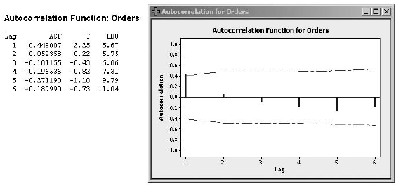
FIGURE 4-22 Autocorrelation Function for Contacts per Order (CPO)
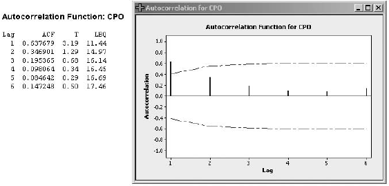
What did Pat and his team learn about the data patterns for orders and contacts per order from the time series plots and autocorrelation functions?
Example 1.2 introduced Pat Niebuhr and his team, who are responsible for developing a global staffing plan for the contact centers of a large web retailer. Pat needs to take a monthly forecast of the total orders and contacts per order (CPO) supplied by the finance department and ultimately forecast the number of customer contacts (phone, email, and so forth) arriving at the retailer's contact centers weekly. The contact centers are open 24 hours 7 days a week and must be appropriately staffed to maintain a high service level. The retailer recognizes that excellent customer service will likely result in repeat visits and purchases.
The key equation for Pat and his team is
Contacts = Orders × CPO
Historical data provide the percentage of contacts for each day of the week. For example, historically 9.10% of the weekly contacts occur on Sundays, 17.25% of the weekly contacts occur on Mondays, and so forth. Keeping in mind the number of Sundays, Mondays, and so on in a given month, monthly forecasts of contacts can be converted to weekly forecasts of contacts. It is the weekly forecasts that are used for staff planning purposes.
Pat thinks it might be a good idea to use the historical data to generate forecasts of orders and contacts per order directly. He is interested in determining whether these forecasts are more accurate than the forecasts for these quantities that the finance department derives from revenue projections. As a start, Pat and his team are interested in the data patterns of the monthly historical orders and contacts per order and decide to plot these time series and analyze the autocorrelations. The data are given in Table 4-12 and plotted in Figures 4-19 and 4-20. The autocorrelations are shown in Figures 4-21 and 4-22.
Pat is intrigued with the time series plots and the autocorrelation functions and feels a smoothing procedure might be the right tool for fitting the time series for orders and contacts per order and for generating forecasts.
TABLE 4-12 Orders and Contacts per Order (CPO) for Web Retailer, June 2001-June 2003
FIGURE 4-19 Time Series Plot of Orders, June 2001-June 2003
FIGURE 4-20 Time Series Plot of Contacts per Order (CPO), June 2001-June 2003
FIGURE 4-21 Autocorrelation Function for Orders
FIGURE 4-22 Autocorrelation Function for Contacts per Order (CPO)
What did Pat and his team learn about the data patterns for orders and contacts per order from the time series plots and autocorrelation functions?
Question
WEB RETAILER
Example 1.2 introduced Pat Niebuhr and his team, who are responsible for developing a global staffing plan for the contact centers of a large web retailer. Pat needs to take a monthly forecast of the total orders and contacts per order (CPO) supplied by the finance department and ultimately forecast the number of customer contacts (phone, email, and so forth) arriving at the retailer's contact centers weekly. The contact centers are open 24 hours 7 days a week and must be appropriately staffed to maintain a high service level. The retailer recognizes that excellent customer service will likely result in repeat visits and purchases.
The key equation for Pat and his team is
Contacts = Orders × CPO
Historical data provide the percentage of contacts for each day of the week. For example, historically 9.10% of the weekly contacts occur on Sundays, 17.25% of the weekly contacts occur on Mondays, and so forth. Keeping in mind the number of Sundays, Mondays, and so on in a given month, monthly forecasts of contacts can be converted to weekly forecasts of contacts. It is the weekly forecasts that are used for staff planning purposes.
Pat thinks it might be a good idea to use the historical data to generate forecasts of orders and contacts per order directly. He is interested in determining whether these forecasts are more accurate than the forecasts for these quantities that the finance department derives from revenue projections. As a start, Pat and his team are interested in the data patterns of the monthly historical orders and contacts per order and decide to plot these time series and analyze the autocorrelations. The data are given in Table 4-12 and plotted in Figures 4-19 and 4-20. The autocorrelations are shown in Figures 4-21 and 4-22.
Pat is intrigued with the time series plots and the autocorrelation functions and feels a smoothing procedure might be the right tool for fitting the time series for orders and contacts per order and for generating forecasts.
TABLE 4-12 Orders and Contacts per Order (CPO) for Web Retailer, June 2001-June 2003

FIGURE 4-19 Time Series Plot of Orders, June 2001-June 2003

FIGURE 4-20 Time Series Plot of Contacts per Order (CPO), June 2001-June 2003
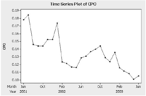
FIGURE 4-21 Autocorrelation Function for Orders

FIGURE 4-22 Autocorrelation Function for Contacts per Order (CPO)

Fit an appropriate smoothing procedure to the orders time series and generate forecasts for the next four months. Justify your choice.
Example 1.2 introduced Pat Niebuhr and his team, who are responsible for developing a global staffing plan for the contact centers of a large web retailer. Pat needs to take a monthly forecast of the total orders and contacts per order (CPO) supplied by the finance department and ultimately forecast the number of customer contacts (phone, email, and so forth) arriving at the retailer's contact centers weekly. The contact centers are open 24 hours 7 days a week and must be appropriately staffed to maintain a high service level. The retailer recognizes that excellent customer service will likely result in repeat visits and purchases.
The key equation for Pat and his team is
Contacts = Orders × CPO
Historical data provide the percentage of contacts for each day of the week. For example, historically 9.10% of the weekly contacts occur on Sundays, 17.25% of the weekly contacts occur on Mondays, and so forth. Keeping in mind the number of Sundays, Mondays, and so on in a given month, monthly forecasts of contacts can be converted to weekly forecasts of contacts. It is the weekly forecasts that are used for staff planning purposes.
Pat thinks it might be a good idea to use the historical data to generate forecasts of orders and contacts per order directly. He is interested in determining whether these forecasts are more accurate than the forecasts for these quantities that the finance department derives from revenue projections. As a start, Pat and his team are interested in the data patterns of the monthly historical orders and contacts per order and decide to plot these time series and analyze the autocorrelations. The data are given in Table 4-12 and plotted in Figures 4-19 and 4-20. The autocorrelations are shown in Figures 4-21 and 4-22.
Pat is intrigued with the time series plots and the autocorrelation functions and feels a smoothing procedure might be the right tool for fitting the time series for orders and contacts per order and for generating forecasts.
TABLE 4-12 Orders and Contacts per Order (CPO) for Web Retailer, June 2001-June 2003
FIGURE 4-19 Time Series Plot of Orders, June 2001-June 2003
FIGURE 4-20 Time Series Plot of Contacts per Order (CPO), June 2001-June 2003
FIGURE 4-21 Autocorrelation Function for Orders
FIGURE 4-22 Autocorrelation Function for Contacts per Order (CPO)
Fit an appropriate smoothing procedure to the orders time series and generate forecasts for the next four months. Justify your choice.
Question
WEB RETAILER
Example 1.2 introduced Pat Niebuhr and his team, who are responsible for developing a global staffing plan for the contact centers of a large web retailer. Pat needs to take a monthly forecast of the total orders and contacts per order (CPO) supplied by the finance department and ultimately forecast the number of customer contacts (phone, email, and so forth) arriving at the retailer's contact centers weekly. The contact centers are open 24 hours 7 days a week and must be appropriately staffed to maintain a high service level. The retailer recognizes that excellent customer service will likely result in repeat visits and purchases.
The key equation for Pat and his team is
Contacts = Orders × CPO
Historical data provide the percentage of contacts for each day of the week. For example, historically 9.10% of the weekly contacts occur on Sundays, 17.25% of the weekly contacts occur on Mondays, and so forth. Keeping in mind the number of Sundays, Mondays, and so on in a given month, monthly forecasts of contacts can be converted to weekly forecasts of contacts. It is the weekly forecasts that are used for staff planning purposes.
Pat thinks it might be a good idea to use the historical data to generate forecasts of orders and contacts per order directly. He is interested in determining whether these forecasts are more accurate than the forecasts for these quantities that the finance department derives from revenue projections. As a start, Pat and his team are interested in the data patterns of the monthly historical orders and contacts per order and decide to plot these time series and analyze the autocorrelations. The data are given in Table 4-12 and plotted in Figures 4-19 and 4-20. The autocorrelations are shown in Figures 4-21 and 4-22.
Pat is intrigued with the time series plots and the autocorrelation functions and feels a smoothing procedure might be the right tool for fitting the time series for orders and contacts per order and for generating forecasts.
TABLE 4-12 Orders and Contacts per Order (CPO) for Web Retailer, June 2001-June 2003

FIGURE 4-19 Time Series Plot of Orders, June 2001-June 2003

FIGURE 4-20 Time Series Plot of Contacts per Order (CPO), June 2001-June 2003

FIGURE 4-21 Autocorrelation Function for Orders

FIGURE 4-22 Autocorrelation Function for Contacts per Order (CPO)

Fit an appropriate smoothing procedure to the contacts per order time series and generate forecasts for the next four months. Justify your choice.
Example 1.2 introduced Pat Niebuhr and his team, who are responsible for developing a global staffing plan for the contact centers of a large web retailer. Pat needs to take a monthly forecast of the total orders and contacts per order (CPO) supplied by the finance department and ultimately forecast the number of customer contacts (phone, email, and so forth) arriving at the retailer's contact centers weekly. The contact centers are open 24 hours 7 days a week and must be appropriately staffed to maintain a high service level. The retailer recognizes that excellent customer service will likely result in repeat visits and purchases.
The key equation for Pat and his team is
Contacts = Orders × CPO
Historical data provide the percentage of contacts for each day of the week. For example, historically 9.10% of the weekly contacts occur on Sundays, 17.25% of the weekly contacts occur on Mondays, and so forth. Keeping in mind the number of Sundays, Mondays, and so on in a given month, monthly forecasts of contacts can be converted to weekly forecasts of contacts. It is the weekly forecasts that are used for staff planning purposes.
Pat thinks it might be a good idea to use the historical data to generate forecasts of orders and contacts per order directly. He is interested in determining whether these forecasts are more accurate than the forecasts for these quantities that the finance department derives from revenue projections. As a start, Pat and his team are interested in the data patterns of the monthly historical orders and contacts per order and decide to plot these time series and analyze the autocorrelations. The data are given in Table 4-12 and plotted in Figures 4-19 and 4-20. The autocorrelations are shown in Figures 4-21 and 4-22.
Pat is intrigued with the time series plots and the autocorrelation functions and feels a smoothing procedure might be the right tool for fitting the time series for orders and contacts per order and for generating forecasts.
TABLE 4-12 Orders and Contacts per Order (CPO) for Web Retailer, June 2001-June 2003
FIGURE 4-19 Time Series Plot of Orders, June 2001-June 2003
FIGURE 4-20 Time Series Plot of Contacts per Order (CPO), June 2001-June 2003
FIGURE 4-21 Autocorrelation Function for Orders
FIGURE 4-22 Autocorrelation Function for Contacts per Order (CPO)
Fit an appropriate smoothing procedure to the contacts per order time series and generate forecasts for the next four months. Justify your choice.
Question
WEB RETAILER
Example 1.2 introduced Pat Niebuhr and his team, who are responsible for developing a global staffing plan for the contact centers of a large web retailer. Pat needs to take a monthly forecast of the total orders and contacts per order (CPO) supplied by the finance department and ultimately forecast the number of customer contacts (phone, email, and so forth) arriving at the retailer's contact centers weekly. The contact centers are open 24 hours 7 days a week and must be appropriately staffed to maintain a high service level. The retailer recognizes that excellent customer service will likely result in repeat visits and purchases.
The key equation for Pat and his team is
Contacts = Orders × CPO
Historical data provide the percentage of contacts for each day of the week. For example, historically 9.10% of the weekly contacts occur on Sundays, 17.25% of the weekly contacts occur on Mondays, and so forth. Keeping in mind the number of Sundays, Mondays, and so on in a given month, monthly forecasts of contacts can be converted to weekly forecasts of contacts. It is the weekly forecasts that are used for staff planning purposes.
Pat thinks it might be a good idea to use the historical data to generate forecasts of orders and contacts per order directly. He is interested in determining whether these forecasts are more accurate than the forecasts for these quantities that the finance department derives from revenue projections. As a start, Pat and his team are interested in the data patterns of the monthly historical orders and contacts per order and decide to plot these time series and analyze the autocorrelations. The data are given in Table 4-12 and plotted in Figures 4-19 and 4-20. The autocorrelations are shown in Figures 4-21 and 4-22.
Pat is intrigued with the time series plots and the autocorrelation functions and feels a smoothing procedure might be the right tool for fitting the time series for orders and contacts per order and for generating forecasts.
TABLE 4-12 Orders and Contacts per Order (CPO) for Web Retailer, June 2001-June 2003

FIGURE 4-19 Time Series Plot of Orders, June 2001-June 2003
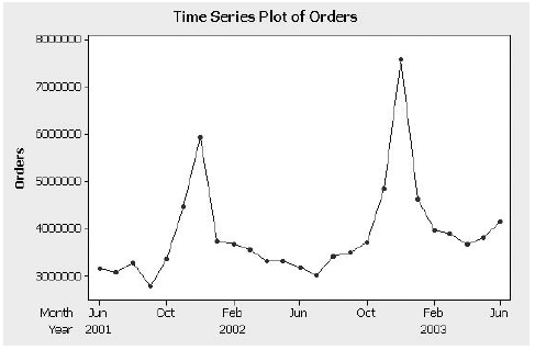
FIGURE 4-20 Time Series Plot of Contacts per Order (CPO), June 2001-June 2003

FIGURE 4-21 Autocorrelation Function for Orders

FIGURE 4-22 Autocorrelation Function for Contacts per Order (CPO)

Use the results for Questions 2 and 3 to generate forecasts of contacts for the next four months.
Example 1.2 introduced Pat Niebuhr and his team, who are responsible for developing a global staffing plan for the contact centers of a large web retailer. Pat needs to take a monthly forecast of the total orders and contacts per order (CPO) supplied by the finance department and ultimately forecast the number of customer contacts (phone, email, and so forth) arriving at the retailer's contact centers weekly. The contact centers are open 24 hours 7 days a week and must be appropriately staffed to maintain a high service level. The retailer recognizes that excellent customer service will likely result in repeat visits and purchases.
The key equation for Pat and his team is
Contacts = Orders × CPO
Historical data provide the percentage of contacts for each day of the week. For example, historically 9.10% of the weekly contacts occur on Sundays, 17.25% of the weekly contacts occur on Mondays, and so forth. Keeping in mind the number of Sundays, Mondays, and so on in a given month, monthly forecasts of contacts can be converted to weekly forecasts of contacts. It is the weekly forecasts that are used for staff planning purposes.
Pat thinks it might be a good idea to use the historical data to generate forecasts of orders and contacts per order directly. He is interested in determining whether these forecasts are more accurate than the forecasts for these quantities that the finance department derives from revenue projections. As a start, Pat and his team are interested in the data patterns of the monthly historical orders and contacts per order and decide to plot these time series and analyze the autocorrelations. The data are given in Table 4-12 and plotted in Figures 4-19 and 4-20. The autocorrelations are shown in Figures 4-21 and 4-22.
Pat is intrigued with the time series plots and the autocorrelation functions and feels a smoothing procedure might be the right tool for fitting the time series for orders and contacts per order and for generating forecasts.
TABLE 4-12 Orders and Contacts per Order (CPO) for Web Retailer, June 2001-June 2003
FIGURE 4-19 Time Series Plot of Orders, June 2001-June 2003
FIGURE 4-20 Time Series Plot of Contacts per Order (CPO), June 2001-June 2003
FIGURE 4-21 Autocorrelation Function for Orders
FIGURE 4-22 Autocorrelation Function for Contacts per Order (CPO)
Use the results for Questions 2 and 3 to generate forecasts of contacts for the next four months.
Question
WEB RETAILER
Example 1.2 introduced Pat Niebuhr and his team, who are responsible for developing a global staffing plan for the contact centers of a large web retailer. Pat needs to take a monthly forecast of the total orders and contacts per order (CPO) supplied by the finance department and ultimately forecast the number of customer contacts (phone, email, and so forth) arriving at the retailer's contact centers weekly. The contact centers are open 24 hours 7 days a week and must be appropriately staffed to maintain a high service level. The retailer recognizes that excellent customer service will likely result in repeat visits and purchases.
The key equation for Pat and his team is
Contacts = Orders × CPO
Historical data provide the percentage of contacts for each day of the week. For example, historically 9.10% of the weekly contacts occur on Sundays, 17.25% of the weekly contacts occur on Mondays, and so forth. Keeping in mind the number of Sundays, Mondays, and so on in a given month, monthly forecasts of contacts can be converted to weekly forecasts of contacts. It is the weekly forecasts that are used for staff planning purposes.
Pat thinks it might be a good idea to use the historical data to generate forecasts of orders and contacts per order directly. He is interested in determining whether these forecasts are more accurate than the forecasts for these quantities that the finance department derives from revenue projections. As a start, Pat and his team are interested in the data patterns of the monthly historical orders and contacts per order and decide to plot these time series and analyze the autocorrelations. The data are given in Table 4-12 and plotted in Figures 4-19 and 4-20. The autocorrelations are shown in Figures 4-21 and 4-22.
Pat is intrigued with the time series plots and the autocorrelation functions and feels a smoothing procedure might be the right tool for fitting the time series for orders and contacts per order and for generating forecasts.
TABLE 4-12 Orders and Contacts per Order (CPO) for Web Retailer, June 2001-June 2003

FIGURE 4-19 Time Series Plot of Orders, June 2001-June 2003

FIGURE 4-20 Time Series Plot of Contacts per Order (CPO), June 2001-June 2003

FIGURE 4-21 Autocorrelation Function for Orders

FIGURE 4-22 Autocorrelation Function for Contacts per Order (CPO)

Pat has access to a spreadsheet with historical actual contacts. He is considering forecasting contacts directly instead of multiplying forecasts of orders and contacts per order to get a forecast. Does this seem reasonable? Why?
Example 1.2 introduced Pat Niebuhr and his team, who are responsible for developing a global staffing plan for the contact centers of a large web retailer. Pat needs to take a monthly forecast of the total orders and contacts per order (CPO) supplied by the finance department and ultimately forecast the number of customer contacts (phone, email, and so forth) arriving at the retailer's contact centers weekly. The contact centers are open 24 hours 7 days a week and must be appropriately staffed to maintain a high service level. The retailer recognizes that excellent customer service will likely result in repeat visits and purchases.
The key equation for Pat and his team is
Contacts = Orders × CPO
Historical data provide the percentage of contacts for each day of the week. For example, historically 9.10% of the weekly contacts occur on Sundays, 17.25% of the weekly contacts occur on Mondays, and so forth. Keeping in mind the number of Sundays, Mondays, and so on in a given month, monthly forecasts of contacts can be converted to weekly forecasts of contacts. It is the weekly forecasts that are used for staff planning purposes.
Pat thinks it might be a good idea to use the historical data to generate forecasts of orders and contacts per order directly. He is interested in determining whether these forecasts are more accurate than the forecasts for these quantities that the finance department derives from revenue projections. As a start, Pat and his team are interested in the data patterns of the monthly historical orders and contacts per order and decide to plot these time series and analyze the autocorrelations. The data are given in Table 4-12 and plotted in Figures 4-19 and 4-20. The autocorrelations are shown in Figures 4-21 and 4-22.
Pat is intrigued with the time series plots and the autocorrelation functions and feels a smoothing procedure might be the right tool for fitting the time series for orders and contacts per order and for generating forecasts.
TABLE 4-12 Orders and Contacts per Order (CPO) for Web Retailer, June 2001-June 2003
FIGURE 4-19 Time Series Plot of Orders, June 2001-June 2003
FIGURE 4-20 Time Series Plot of Contacts per Order (CPO), June 2001-June 2003
FIGURE 4-21 Autocorrelation Function for Orders
FIGURE 4-22 Autocorrelation Function for Contacts per Order (CPO)
Pat has access to a spreadsheet with historical actual contacts. He is considering forecasting contacts directly instead of multiplying forecasts of orders and contacts per order to get a forecast. Does this seem reasonable? Why?
Question
WEB RETAILER
Example 1.2 introduced Pat Niebuhr and his team, who are responsible for developing a global staffing plan for the contact centers of a large web retailer. Pat needs to take a monthly forecast of the total orders and contacts per order (CPO) supplied by the finance department and ultimately forecast the number of customer contacts (phone, email, and so forth) arriving at the retailer's contact centers weekly. The contact centers are open 24 hours 7 days a week and must be appropriately staffed to maintain a high service level. The retailer recognizes that excellent customer service will likely result in repeat visits and purchases.
The key equation for Pat and his team is
Contacts = Orders × CPO
Historical data provide the percentage of contacts for each day of the week. For example, historically 9.10% of the weekly contacts occur on Sundays, 17.25% of the weekly contacts occur on Mondays, and so forth. Keeping in mind the number of Sundays, Mondays, and so on in a given month, monthly forecasts of contacts can be converted to weekly forecasts of contacts. It is the weekly forecasts that are used for staff planning purposes.
Pat thinks it might be a good idea to use the historical data to generate forecasts of orders and contacts per order directly. He is interested in determining whether these forecasts are more accurate than the forecasts for these quantities that the finance department derives from revenue projections. As a start, Pat and his team are interested in the data patterns of the monthly historical orders and contacts per order and decide to plot these time series and analyze the autocorrelations. The data are given in Table 4-12 and plotted in Figures 4-19 and 4-20. The autocorrelations are shown in Figures 4-21 and 4-22.
Pat is intrigued with the time series plots and the autocorrelation functions and feels a smoothing procedure might be the right tool for fitting the time series for orders and contacts per order and for generating forecasts.
TABLE 4-12 Orders and Contacts per Order (CPO) for Web Retailer, June 2001-June 2003
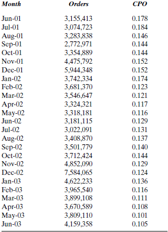
FIGURE 4-19 Time Series Plot of Orders, June 2001-June 2003

FIGURE 4-20 Time Series Plot of Contacts per Order (CPO), June 2001-June 2003

FIGURE 4-21 Autocorrelation Function for Orders

FIGURE 4-22 Autocorrelation Function for Contacts per Order (CPO)

Many orders consist of more than one item (unit). Would it be better to focus on number of units and contacts per unit to get a forecast of contacts? Discuss.
Example 1.2 introduced Pat Niebuhr and his team, who are responsible for developing a global staffing plan for the contact centers of a large web retailer. Pat needs to take a monthly forecast of the total orders and contacts per order (CPO) supplied by the finance department and ultimately forecast the number of customer contacts (phone, email, and so forth) arriving at the retailer's contact centers weekly. The contact centers are open 24 hours 7 days a week and must be appropriately staffed to maintain a high service level. The retailer recognizes that excellent customer service will likely result in repeat visits and purchases.
The key equation for Pat and his team is
Contacts = Orders × CPO
Historical data provide the percentage of contacts for each day of the week. For example, historically 9.10% of the weekly contacts occur on Sundays, 17.25% of the weekly contacts occur on Mondays, and so forth. Keeping in mind the number of Sundays, Mondays, and so on in a given month, monthly forecasts of contacts can be converted to weekly forecasts of contacts. It is the weekly forecasts that are used for staff planning purposes.
Pat thinks it might be a good idea to use the historical data to generate forecasts of orders and contacts per order directly. He is interested in determining whether these forecasts are more accurate than the forecasts for these quantities that the finance department derives from revenue projections. As a start, Pat and his team are interested in the data patterns of the monthly historical orders and contacts per order and decide to plot these time series and analyze the autocorrelations. The data are given in Table 4-12 and plotted in Figures 4-19 and 4-20. The autocorrelations are shown in Figures 4-21 and 4-22.
Pat is intrigued with the time series plots and the autocorrelation functions and feels a smoothing procedure might be the right tool for fitting the time series for orders and contacts per order and for generating forecasts.
TABLE 4-12 Orders and Contacts per Order (CPO) for Web Retailer, June 2001-June 2003
FIGURE 4-19 Time Series Plot of Orders, June 2001-June 2003
FIGURE 4-20 Time Series Plot of Contacts per Order (CPO), June 2001-June 2003
FIGURE 4-21 Autocorrelation Function for Orders
FIGURE 4-22 Autocorrelation Function for Contacts per Order (CPO)
Many orders consist of more than one item (unit). Would it be better to focus on number of units and contacts per unit to get a forecast of contacts? Discuss.
Question
SOUTHWEST MEDICAL CENTER
Mary Beasley is responsible for keeping track of the number of billable visits to the Medical Oncology group at Southwest Medical Center. Her anecdotal evidence suggests that the number of visits has been increasing and some parts of the year seem to be busier than others. Some doctors are beginning to complain about the work load and suggest they don't always have enough time to interact with individual patients. Will additional medical staff be required to handle the apparently increasing demand?
If so, how many new doctors should be hired and/or be reassigned from other areas?
To provide some insight into the nature of the demand for service, Mary opens her Excel spreadsheet and examines the total number of billable visits on a monthly basis for the last several fiscal years. The data are listed in Table 4-13.
A time series plot of Mary's data is shown in Figure 4-23. As expected, the time series shows an upward trend, but Mary is not sure if there is a seasonal component in the total visits series. She decides to investigate this issue by constructing the autocorrelation function. If a seasonal component exists with monthly data, Mary expects to see fairly large autocorrelations at the seasonal lags: 12, 24, and so forth. Mary knows from a course in her Executive MBA program that Winters' smoothing procedure might be a good way to generate forecasts of future visits if trend and seasonal components are present.
TABLE 4-13 Total Billable Visits to Medical Oncology, FY1995-FY2004

FIGURE 4-23 Time Series Plot of Total Visits to Medical Oncology, FY1995-FY2004

What did Mary's autocorrelation analysis show?
Mary Beasley is responsible for keeping track of the number of billable visits to the Medical Oncology group at Southwest Medical Center. Her anecdotal evidence suggests that the number of visits has been increasing and some parts of the year seem to be busier than others. Some doctors are beginning to complain about the work load and suggest they don't always have enough time to interact with individual patients. Will additional medical staff be required to handle the apparently increasing demand?
If so, how many new doctors should be hired and/or be reassigned from other areas?
To provide some insight into the nature of the demand for service, Mary opens her Excel spreadsheet and examines the total number of billable visits on a monthly basis for the last several fiscal years. The data are listed in Table 4-13.
A time series plot of Mary's data is shown in Figure 4-23. As expected, the time series shows an upward trend, but Mary is not sure if there is a seasonal component in the total visits series. She decides to investigate this issue by constructing the autocorrelation function. If a seasonal component exists with monthly data, Mary expects to see fairly large autocorrelations at the seasonal lags: 12, 24, and so forth. Mary knows from a course in her Executive MBA program that Winters' smoothing procedure might be a good way to generate forecasts of future visits if trend and seasonal components are present.
TABLE 4-13 Total Billable Visits to Medical Oncology, FY1995-FY2004
FIGURE 4-23 Time Series Plot of Total Visits to Medical Oncology, FY1995-FY2004
What did Mary's autocorrelation analysis show?
Question
SOUTHWEST MEDICAL CENTER
Mary Beasley is responsible for keeping track of the number of billable visits to the Medical Oncology group at Southwest Medical Center. Her anecdotal evidence suggests that the number of visits has been increasing and some parts of the year seem to be busier than others. Some doctors are beginning to complain about the work load and suggest they don't always have enough time to interact with individual patients. Will additional medical staff be required to handle the apparently increasing demand?
If so, how many new doctors should be hired and/or be reassigned from other areas?
To provide some insight into the nature of the demand for service, Mary opens her Excel spreadsheet and examines the total number of billable visits on a monthly basis for the last several fiscal years. The data are listed in Table 4-13.
A time series plot of Mary's data is shown in Figure 4-23. As expected, the time series shows an upward trend, but Mary is not sure if there is a seasonal component in the total visits series. She decides to investigate this issue by constructing the autocorrelation function. If a seasonal component exists with monthly data, Mary expects to see fairly large autocorrelations at the seasonal lags: 12, 24, and so forth. Mary knows from a course in her Executive MBA program that Winters' smoothing procedure might be a good way to generate forecasts of future visits if trend and seasonal components are present.
TABLE 4-13 Total Billable Visits to Medical Oncology, FY1995-FY2004

FIGURE 4-23 Time Series Plot of Total Visits to Medical Oncology, FY1995-FY2004

Fit an appropriate smoothing procedure to Mary's data, examine the residual autocorrelations, and generate forecasts for the remainder of FY2003-04. Do these forecasts seem reasonable?
Mary Beasley is responsible for keeping track of the number of billable visits to the Medical Oncology group at Southwest Medical Center. Her anecdotal evidence suggests that the number of visits has been increasing and some parts of the year seem to be busier than others. Some doctors are beginning to complain about the work load and suggest they don't always have enough time to interact with individual patients. Will additional medical staff be required to handle the apparently increasing demand?
If so, how many new doctors should be hired and/or be reassigned from other areas?
To provide some insight into the nature of the demand for service, Mary opens her Excel spreadsheet and examines the total number of billable visits on a monthly basis for the last several fiscal years. The data are listed in Table 4-13.
A time series plot of Mary's data is shown in Figure 4-23. As expected, the time series shows an upward trend, but Mary is not sure if there is a seasonal component in the total visits series. She decides to investigate this issue by constructing the autocorrelation function. If a seasonal component exists with monthly data, Mary expects to see fairly large autocorrelations at the seasonal lags: 12, 24, and so forth. Mary knows from a course in her Executive MBA program that Winters' smoothing procedure might be a good way to generate forecasts of future visits if trend and seasonal components are present.
TABLE 4-13 Total Billable Visits to Medical Oncology, FY1995-FY2004
FIGURE 4-23 Time Series Plot of Total Visits to Medical Oncology, FY1995-FY2004
Fit an appropriate smoothing procedure to Mary's data, examine the residual autocorrelations, and generate forecasts for the remainder of FY2003-04. Do these forecasts seem reasonable?
Question
SOUTHWEST MEDICAL CENTER
Mary Beasley is responsible for keeping track of the number of billable visits to the Medical Oncology group at Southwest Medical Center. Her anecdotal evidence suggests that the number of visits has been increasing and some parts of the year seem to be busier than others. Some doctors are beginning to complain about the work load and suggest they don't always have enough time to interact with individual patients. Will additional medical staff be required to handle the apparently increasing demand?
If so, how many new doctors should be hired and/or be reassigned from other areas?
To provide some insight into the nature of the demand for service, Mary opens her Excel spreadsheet and examines the total number of billable visits on a monthly basis for the last several fiscal years. The data are listed in Table 4-13.
A time series plot of Mary's data is shown in Figure 4-23. As expected, the time series shows an upward trend, but Mary is not sure if there is a seasonal component in the total visits series. She decides to investigate this issue by constructing the autocorrelation function. If a seasonal component exists with monthly data, Mary expects to see fairly large autocorrelations at the seasonal lags: 12, 24, and so forth. Mary knows from a course in her Executive MBA program that Winters' smoothing procedure might be a good way to generate forecasts of future visits if trend and seasonal components are present.
TABLE 4-13 Total Billable Visits to Medical Oncology, FY1995-FY2004
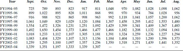
FIGURE 4-23 Time Series Plot of Total Visits to Medical Oncology, FY1995-FY2004
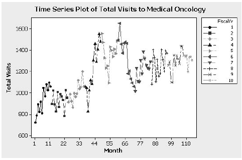
Given the results in Question 2, do you think it is likely another forecasting method would generate "better" forecasts? Discuss.
Mary Beasley is responsible for keeping track of the number of billable visits to the Medical Oncology group at Southwest Medical Center. Her anecdotal evidence suggests that the number of visits has been increasing and some parts of the year seem to be busier than others. Some doctors are beginning to complain about the work load and suggest they don't always have enough time to interact with individual patients. Will additional medical staff be required to handle the apparently increasing demand?
If so, how many new doctors should be hired and/or be reassigned from other areas?
To provide some insight into the nature of the demand for service, Mary opens her Excel spreadsheet and examines the total number of billable visits on a monthly basis for the last several fiscal years. The data are listed in Table 4-13.
A time series plot of Mary's data is shown in Figure 4-23. As expected, the time series shows an upward trend, but Mary is not sure if there is a seasonal component in the total visits series. She decides to investigate this issue by constructing the autocorrelation function. If a seasonal component exists with monthly data, Mary expects to see fairly large autocorrelations at the seasonal lags: 12, 24, and so forth. Mary knows from a course in her Executive MBA program that Winters' smoothing procedure might be a good way to generate forecasts of future visits if trend and seasonal components are present.
TABLE 4-13 Total Billable Visits to Medical Oncology, FY1995-FY2004
FIGURE 4-23 Time Series Plot of Total Visits to Medical Oncology, FY1995-FY2004
Given the results in Question 2, do you think it is likely another forecasting method would generate "better" forecasts? Discuss.
Question
SOUTHWEST MEDICAL CENTER
Mary Beasley is responsible for keeping track of the number of billable visits to the Medical Oncology group at Southwest Medical Center. Her anecdotal evidence suggests that the number of visits has been increasing and some parts of the year seem to be busier than others. Some doctors are beginning to complain about the work load and suggest they don't always have enough time to interact with individual patients. Will additional medical staff be required to handle the apparently increasing demand?
If so, how many new doctors should be hired and/or be reassigned from other areas?
To provide some insight into the nature of the demand for service, Mary opens her Excel spreadsheet and examines the total number of billable visits on a monthly basis for the last several fiscal years. The data are listed in Table 4-13.
A time series plot of Mary's data is shown in Figure 4-23. As expected, the time series shows an upward trend, but Mary is not sure if there is a seasonal component in the total visits series. She decides to investigate this issue by constructing the autocorrelation function. If a seasonal component exists with monthly data, Mary expects to see fairly large autocorrelations at the seasonal lags: 12, 24, and so forth. Mary knows from a course in her Executive MBA program that Winters' smoothing procedure might be a good way to generate forecasts of future visits if trend and seasonal components are present.
TABLE 4-13 Total Billable Visits to Medical Oncology, FY1995-FY2004

FIGURE 4-23 Time Series Plot of Total Visits to Medical Oncology, FY1995-FY2004

Do you think additional medical staff might be needed to handle future demand? Write a brief report summarizing Mary's data analysis and the implications for additional staff.
Mary Beasley is responsible for keeping track of the number of billable visits to the Medical Oncology group at Southwest Medical Center. Her anecdotal evidence suggests that the number of visits has been increasing and some parts of the year seem to be busier than others. Some doctors are beginning to complain about the work load and suggest they don't always have enough time to interact with individual patients. Will additional medical staff be required to handle the apparently increasing demand?
If so, how many new doctors should be hired and/or be reassigned from other areas?
To provide some insight into the nature of the demand for service, Mary opens her Excel spreadsheet and examines the total number of billable visits on a monthly basis for the last several fiscal years. The data are listed in Table 4-13.
A time series plot of Mary's data is shown in Figure 4-23. As expected, the time series shows an upward trend, but Mary is not sure if there is a seasonal component in the total visits series. She decides to investigate this issue by constructing the autocorrelation function. If a seasonal component exists with monthly data, Mary expects to see fairly large autocorrelations at the seasonal lags: 12, 24, and so forth. Mary knows from a course in her Executive MBA program that Winters' smoothing procedure might be a good way to generate forecasts of future visits if trend and seasonal components are present.
TABLE 4-13 Total Billable Visits to Medical Oncology, FY1995-FY2004
FIGURE 4-23 Time Series Plot of Total Visits to Medical Oncology, FY1995-FY2004
Do you think additional medical staff might be needed to handle future demand? Write a brief report summarizing Mary's data analysis and the implications for additional staff.
Question
Question
Question
Question

Unlock Deck
Sign up to unlock the cards in this deck!
Unlock Deck
Unlock Deck
1/50
Play
Full screen (f)
Deck 3: Moving Averages and Smoothing Methods
1
Which forecasting technique continually revises an estimate in the light of more-recent experiences?
Identify the forecasting technique.
The Exponential Smoothing forecasting technique continually revises an estimate in the light of more recent experiences.
Explanation:
In the Exponential Smoothing forecasting technique, the exponentially decreasing weights are assigned when the observations get older. Also, in the forecasting more weights are given by the recent observations when compared to the older observations.
2
Which forecasting technique uses the value for the current period as the forecast for the next period?
Identify the forecasting technique.
The Naive forecasting technique uses the value for the current period as the forecast for the next period.
Explanation:
In the Naive forecasting technique, the actual value of the last period is used as the forecast value of this period. In other words, the recent periods are the best predictors of the future. The model is given below,
 Where, the forecast made at time t for time
 is denoted as
 .
.
The Naive forecasting technique uses the value for the current period as the forecast for the next period.
Explanation:
In the Naive forecasting technique, the actual value of the last period is used as the forecast value of this period. In other words, the recent periods are the best predictors of the future. The model is given below,
Where, the forecast made at time t for time is denoted as . 3
Which forecasting technique assigns equal weight to each observation?
Identify the forecasting technique.
The Moving average forecasting technique assigns equal weight to each observation.
Explanation:
In the moving average forecasting technique, the oldest data point is removed and the new data point is included in the average as it becomes available. That is, the weights are assigned equally to each observation. Moreover, the rate of response in the above mentioned data pattern depends upon the number of periods, which is involved in the moving average.
4
Which forecasting technique(s) should be tried if the data are trending?
Unlock Deck
Unlock for access to all 50 flashcards in this deck.
Unlock Deck
k this deck
5
Which forecasting technique(s) should be tried if the data are seasonal?
Unlock Deck
Unlock for access to all 50 flashcards in this deck.
Unlock Deck
k this deck
6
Apex Mutual Fund invests primarily in technology stocks. The price of the fund at the end of each month for the 12 months of 2006 is shown in Table P-6.
a. Find the forecast value of the mutual fund for each month by using a naive model (see Equation 4.1). The value for December 2005 was 19.00.
b. Evaluate this forecasting method using the MAD.
c. Evaluate this forecasting method using the MSE.
d. Evaluate this forecasting method using the MAPE.
e. Evaluate this forecasting method using the MPE.
f. Using a naive model, forecast the mutual fund price for January 2007.
g. Write a memo summarizing your findings.
TABLE P-6
a. Find the forecast value of the mutual fund for each month by using a naive model (see Equation 4.1). The value for December 2005 was 19.00.
b. Evaluate this forecasting method using the MAD.
c. Evaluate this forecasting method using the MSE.
d. Evaluate this forecasting method using the MAPE.
e. Evaluate this forecasting method using the MPE.
f. Using a naive model, forecast the mutual fund price for January 2007.
g. Write a memo summarizing your findings.
TABLE P-6
Unlock Deck
Unlock for access to all 50 flashcards in this deck.
Unlock Deck
k this deck
7
Refer to Problem 6. Use a three-month moving average to forecast the mutual fund price for January 2007. Is this forecast better than the forecast made using the naive model? Explain.
Unlock Deck
Unlock for access to all 50 flashcards in this deck.
Unlock Deck
k this deck
8
Given the series Y t in Table P-8:
a. What is the forecast for period 9, using a five-period moving average?
b. If simple exponential smoothing with a smoothing constant of.4 is used, what is the forecast for time period 4?
c. In part b, what is the forecast error for time period 3?
TABLE P-8
a. What is the forecast for period 9, using a five-period moving average?
b. If simple exponential smoothing with a smoothing constant of.4 is used, what is the forecast for time period 4?
c. In part b, what is the forecast error for time period 3?
TABLE P-8
Unlock Deck
Unlock for access to all 50 flashcards in this deck.
Unlock Deck
k this deck
9
The yield on a general obligation bond for the city of Davenport fluctuates with the market. The monthly quotations for 2006 are given in Table P-9.
TABLE P-9
a. Find the forecast value of the yield for the obligation bonds for each month, starting with April, using a three-month moving average.
b. Find the forecast value of the yield for the obligation bonds for each month, starting with June, using a five-month moving average.
c. Evaluate these forecasting methods using the MAD.
d. Evaluate these forecasting methods using the MSE.
e. Evaluate these forecasting methods using the MAPE.
f. Evaluate these forecasting methods using the MPE.
g. Forecast the yield for January 2007 using the better technique.
h. Write a memo summarizing your findings.
TABLE P-9
a. Find the forecast value of the yield for the obligation bonds for each month, starting with April, using a three-month moving average.
b. Find the forecast value of the yield for the obligation bonds for each month, starting with June, using a five-month moving average.
c. Evaluate these forecasting methods using the MAD.
d. Evaluate these forecasting methods using the MSE.
e. Evaluate these forecasting methods using the MAPE.
f. Evaluate these forecasting methods using the MPE.
g. Forecast the yield for January 2007 using the better technique.
h. Write a memo summarizing your findings.
Unlock Deck
Unlock for access to all 50 flashcards in this deck.
Unlock Deck
k this deck
10
This question refers to Problem 9. Use exponential smoothing with a smoothing constant of.2 and an initial value of 9.29 to forecast the yield for January 2007. Is this forecast better than the forecast made using the better moving average model? Explain.
Unlock Deck
Unlock for access to all 50 flashcards in this deck.
Unlock Deck
k this deck
11
The Hughes Supply Company uses an inventory management method to determine the monthly demands for various products. The demand values for the last 12 months of each product have been recorded and are available for future forecasting. The demand values for the 12 months of 2006 for one electrical fixture are presented in Table P-11.
TABLE P-11
Source: Based on Hughes Supply Company records.
Use exponential smoothing with a smoothing constant of.5 and an initial value of 205 to forecast the demand for January 2007.
TABLE P-11
Source: Based on Hughes Supply Company records.
Use exponential smoothing with a smoothing constant of.5 and an initial value of 205 to forecast the demand for January 2007.
Unlock Deck
Unlock for access to all 50 flashcards in this deck.
Unlock Deck
k this deck
12
General American Investors Company, a closed-end regulated investment management company, invests primarily in medium- and high-quality stocks. Jim Campbell is studying the asset value per share for this company and would like to forecast this variable for the remaining quarters of 1996. The data are presented in Table P-12.
Evaluate the ability to forecast the asset value per share variable of the following forecasting methods: naive, moving average, and exponential smoothing. When you compare techniques, take into consideration that the actual asset value per share for the second quarter of 1996 was 26.47. Write a report for Jim indicating which method he should use and why.
TABLE P-12 General American Investors Company Assets per Share, 1985-1996
Source: The Value Line Investment Survey (New York: Value Line, 1990, 1993, 1996).
Unlock Deck
Unlock for access to all 50 flashcards in this deck.
Unlock Deck
k this deck
13
Southdown, Inc., the nation's third largest cement producer, is pushing ahead with a waste fuel burning program. The cost for Southdown will total about $37 million. For this reason, it is extremely important for the company to have an accurate forecast of revenues for the first quarter of 2000. The data are presented in Table P-13.
a. Use exponential smoothing with a smoothing constant of.4 and an initial value of 77.4 to forecast the quarterly revenues for the first quarter of 2000.
b. Now use a smoothing constant of.6 and an initial value of 77.4 to forecast the quarterly revenues for the first quarter of 2000.
c. Which smoothing constant provides the better forecast?
d. Refer to part c. Examine the residual autocorrelations. Are you happy with simple exponential smoothing for this example? Explain.
TABLE P-13 Southdown Revenues, 1986-1999
Source: The Value Line Investment Survey (New York: Value Line, 1990, 1993, 1996, 1999).
Unlock Deck
Unlock for access to all 50 flashcards in this deck.
Unlock Deck
k this deck
14
The Triton Energy Corporation explores for and produces oil and gas. Company president Gail Freeman wants to have her company's analyst forecast the company's sales per share for 2000. This will be an important forecast, since Triton's restructuring plans have hit a snag. The data are presented in Table P-14.
Determine the best forecasting method and forecast sales per share for 2000.
TABLE P-14 Triton Sales per Share, 1974-1999
Source: The Value Line Investment Survey (New York: Value Line, 1990, 1993, 1996, 1999)
Determine the best forecasting method and forecast sales per share for 2000.
TABLE P-14 Triton Sales per Share, 1974-1999
Source: The Value Line Investment Survey (New York: Value Line, 1990, 1993, 1996, 1999)
Unlock Deck
Unlock for access to all 50 flashcards in this deck.
Unlock Deck
k this deck
15
The Consolidated Edison Company sells electricity (82% of revenues), gas (13%), and steam (5%) in New York City and Westchester County. Bart Thomas, company forecaster, is assigned the task of forecasting the company's quarterly revenues for the rest of 2002 and all of 2003. He collects the data shown in Table P-15.
Determine the best forecasting technique and forecast quarterly revenue for the rest of 2002 and all of 2003.
TABLE P-15 Quarterly Revenues for Consolidated Edison ($ millions), 1985-June 2002
Source: The Value Line Investment Survey (New York: Value Line, 1990, 1993, 1996, 1999, 2001).
Determine the best forecasting technique and forecast quarterly revenue for the rest of 2002 and all of 2003.
TABLE P-15 Quarterly Revenues for Consolidated Edison ($ millions), 1985-June 2002
Source: The Value Line Investment Survey (New York: Value Line, 1990, 1993, 1996, 1999, 2001).
Unlock Deck
Unlock for access to all 50 flashcards in this deck.
Unlock Deck
k this deck
16
A job-shop manufacturer that specializes in replacement parts has no forecasting system in place and manufactures products based on last month's sales. Twenty-four months of sales data are available and are given in Table P-16.
a. Plot the sales data as a time series. Are the data seasonal?
Hint: For monthly data, the seasonal period is s = 12. Is there a pattern (e.g., summer sales relatively low, fall sales relatively high) that tends to repeat itself every 12 months?
TABLE P-16
b. Use a naive model to generate monthly sales forecasts (e.g., the February 2005 forecast is given by the January 2005 value, and so forth). Compute the MAPE.
c. Use simple exponential smoothing with a smoothing constant of.5 and an initial smoothed value of 430 to generate sales forecasts for each month. Compute the MAPE.
d. Do you think either of the models in parts b and c is likely to generate accurate forecasts for future monthly sales? Explain.
e. Use Minitab and Winters' multiplicative smoothing method with smoothing constants ? = ? = ? =.5 to generate a forecast for January 2007. Save the residuals.
f. Refer to part e. Compare the MAPE for Winters' method from the computer printout with the MAPE s in parts b and c. Which of the three forecasting procedures do you prefer?
g. Refer to part e. Compute the autocorrelations (for six lags) for the residuals from Winters' multiplicative procedure. Do the residual autocorrelations suggest that Winters' procedure works well for these data? Explain.
a. Plot the sales data as a time series. Are the data seasonal?
Hint: For monthly data, the seasonal period is s = 12. Is there a pattern (e.g., summer sales relatively low, fall sales relatively high) that tends to repeat itself every 12 months?
TABLE P-16
b. Use a naive model to generate monthly sales forecasts (e.g., the February 2005 forecast is given by the January 2005 value, and so forth). Compute the MAPE.
c. Use simple exponential smoothing with a smoothing constant of.5 and an initial smoothed value of 430 to generate sales forecasts for each month. Compute the MAPE.
d. Do you think either of the models in parts b and c is likely to generate accurate forecasts for future monthly sales? Explain.
e. Use Minitab and Winters' multiplicative smoothing method with smoothing constants ? = ? = ? =.5 to generate a forecast for January 2007. Save the residuals.
f. Refer to part e. Compare the MAPE for Winters' method from the computer printout with the MAPE s in parts b and c. Which of the three forecasting procedures do you prefer?
g. Refer to part e. Compute the autocorrelations (for six lags) for the residuals from Winters' multiplicative procedure. Do the residual autocorrelations suggest that Winters' procedure works well for these data? Explain.
Unlock Deck
Unlock for access to all 50 flashcards in this deck.
Unlock Deck
k this deck
17
Consider the gasoline purchases for the Spokane Transit Authority given in Table 4-2. In Example 4.3, a five-week moving average is used to smooth the data and generate forecasts.
a. Use Minitab to smooth the Spokane Transit Authority data using a four-week moving average. Which moving average length, four weeks or five weeks, appears to represent the data better? Explain.
b. Use Minitab to smooth the Spokane Transit Authority data using simple exponential smoothing. Compare your results with those in part a. Which procedure, four-week moving average or simple exponential smoothing, do you prefer for these data? Explain.
Unlock Deck
Unlock for access to all 50 flashcards in this deck.
Unlock Deck
k this deck
18
Table P-18 contains the number of severe earthquakes (those with a Richter scale magnitude of 7 and above) per year for the years 1900-1999.
TABLE P-18 Number of Severe Earthquakes, 1900-1999
Source: U.S. Geological Survey Earthquake Hazard Program.
a. Use Minitab to smooth the earthquake data with moving averages of orders k = 5, 10, and 15. Describe the nature of the smoothing as the order of the moving average increases. Do you think there might be a cycle in these data? If so, provide an estimate of the length (in years) of the cycle.
b. Use Minitab to smooth the earthquake data using simple exponential smoothing. Store the residuals and generate a forecast for the number of severe earthquakes in the year 2000. Compute the residual autocorrelations. Does simple exponential smoothing provide a reasonable fit to these data? Explain.
c. Is there a seasonal component in the earthquake data? Why or why not?
Unlock Deck
Unlock for access to all 50 flashcards in this deck.
Unlock Deck
k this deck
19
Table P-23 in Chapter 3 contains the quarterly income before extraordinary items for Southwest Airlines for the years 1988-1999.
a. Using Minitab, smooth the Southwest Airlines income data using Holt's linear smoothing and store the residuals. Compute the residual autocorrelations. Does it appear as if Holt's smoothing procedure represents these data well? If not, what time series component (trend, cycle, seasonal) is not accounted for by Holt's method?
b. Use Minitab to smooth the Southwest Airlines income data using Winters' multiplicative exponential smoothing. Store the residuals and generate forecasts of income for the four quarters of 2000. Compute the residual autocorrelations. Does Winters' smoothing technique fit the income data well? Do the forecasts seem reasonable? Discuss.
Unlock Deck
Unlock for access to all 50 flashcards in this deck.
Unlock Deck
k this deck
20
Table P-20 contains quarterly sales ($MM) of The Gap for fiscal years 1980-2004.
Plot The Gap sales data as a time series and examine its properties. The objective is to generate forecasts of sales for the four quarters of 2005. Select an appropriate smoothing method for forecasting and justify your choice.
TABLE P-20 Quarterly Sales for The Gap, Fiscal Years 1980-2004
Source: Based on The Value Line Investment Survey (New York: Value Line, various years), and 10K filings with the Securities and Exchange Commission.
Unlock Deck
Unlock for access to all 50 flashcards in this deck.
Unlock Deck
k this deck
21
THE SOLAR ALTERNATIVE COMPANY
The Solar Alternative Company is about to enter its third year of operation. Bob and Mary Johnson, who both teach science in the local high school, founded the company. The Johnsons started the Solar Alternative Company to supplement their teaching income. Based on their research into solar energy systems, they were able to put together a solar system for heating domestic hot water. The system consists of a 100-gallon fiberglass storage tank, two 36-foot solar panels, electronic controls, PVC pipe, and miscellaneous fittings.
The payback period on the system is 10 years. Although this situation does not present an attractive investment opportunity from a financial point of view, there is sufficient interest in the novelty of the concept to provide a moderate level of sales. The Johnsons clear about $75 on the $2,000 price of an installed system, after costs and expenses. Material and equipment costs account for 75% of the installed system cost. An advantage that helps to offset the low profit margin is the fact that the product is not profitable enough to generate any significant competition from heating contractors. The Johnsons operate the business out of their home. They have an office in the basement, and their one-car garage is used exclusively to store the system components and materials. As a result, overhead is at a minimum. The Johnsons enjoy a modest supplemental income from the company's operation. The business also provides a number of tax advantages.
Bob and Mary are pleased with the growth of the business. Although sales vary from month to month, overall the second year was much better than the first. Many of the second-year customers are neighbors of people who had purchased the system in the first year. Apparently, after seeing the system operate successfully for a year, others were willing to try the solar concept. Sales occur throughout the year. Demand for the system is greatest in late summer and early fall, when homeowners typically make plans to winterize their homes for the upcoming heating season.
With the anticipated growth in the business, the Johnsons felt that they needed a sales forecast to manage effectively in the coming year. It usually takes 60 to 90 days to receive storage tanks after placing the order. The solar panels are available off the shelf most of the year. However, in the late summer and throughout the fall, the lead time can be as much as 90 to 100 days. Although there is limited competition, lost sales are nevertheless a real possibility if the potential customer is asked to wait several months for installation. Perhaps more important is the need to make accurate sales projections to take advantage of quantity discount buying. These factors, when combined with the high cost of system components and the limited storage space available in the garage, make it necessary to develop a reliable forecast. The sales history for the company's first two years is given in Table 4-10.
TABLE 4-10
Identify the model Bob and Mary should use as the basis for their business planning in 2007, and discuss why you selected this model.
Unlock Deck
Unlock for access to all 50 flashcards in this deck.
Unlock Deck
k this deck
22
THE SOLAR ALTERNATIVE COMPANY
The Solar Alternative Company is about to enter its third year of operation. Bob and Mary Johnson, who both teach science in the local high school, founded the company. The Johnsons started the Solar Alternative Company to supplement their teaching income. Based on their research into solar energy systems, they were able to put together a solar system for heating domestic hot water. The system consists of a 100-gallon fiberglass storage tank, two 36-foot solar panels, electronic controls, PVC pipe, and miscellaneous fittings.
The payback period on the system is 10 years. Although this situation does not present an attractive investment opportunity from a financial point of view, there is sufficient interest in the novelty of the concept to provide a moderate level of sales. The Johnsons clear about $75 on the $2,000 price of an installed system, after costs and expenses. Material and equipment costs account for 75% of the installed system cost. An advantage that helps to offset the low profit margin is the fact that the product is not profitable enough to generate any significant competition from heating contractors. The Johnsons operate the business out of their home. They have an office in the basement, and their one-car garage is used exclusively to store the system components and materials. As a result, overhead is at a minimum. The Johnsons enjoy a modest supplemental income from the company's operation. The business also provides a number of tax advantages.
Bob and Mary are pleased with the growth of the business. Although sales vary from month to month, overall the second year was much better than the first. Many of the second-year customers are neighbors of people who had purchased the system in the first year. Apparently, after seeing the system operate successfully for a year, others were willing to try the solar concept. Sales occur throughout the year. Demand for the system is greatest in late summer and early fall, when homeowners typically make plans to winterize their homes for the upcoming heating season.
With the anticipated growth in the business, the Johnsons felt that they needed a sales forecast to manage effectively in the coming year. It usually takes 60 to 90 days to receive storage tanks after placing the order. The solar panels are available off the shelf most of the year. However, in the late summer and throughout the fall, the lead time can be as much as 90 to 100 days. Although there is limited competition, lost sales are nevertheless a real possibility if the potential customer is asked to wait several months for installation. Perhaps more important is the need to make accurate sales projections to take advantage of quantity discount buying. These factors, when combined with the high cost of system components and the limited storage space available in the garage, make it necessary to develop a reliable forecast. The sales history for the company's first two years is given in Table 4-10.
TABLE 4-10
Forecast sales for 2007.
Unlock Deck
Unlock for access to all 50 flashcards in this deck.
Unlock Deck
k this deck
23
TUX
John Mosby, owner of several Mr. Tux rental stores, is beginning to forecast his most important business variable, monthly dollar sales (see the Mr. Tux cases in previous chapters). One of his employees, Virginia Perot, gathered the sales data shown in Case 2-2. John now wants to create a forecast based on these sales data using moving average and exponential smoothing techniques.
John used Minitab in Case 3-2 to determine that these data are both trending and seasonal. He has been told that simple moving averages and exponential smoothing techniques will not work with these data but decides to find out for himself.
He begins by trying a three-month moving average. The program calculates several summary forecast error measurements. These values summarize the errors found in predicting actual historical data values using a three-month moving average. John decides to record two of these error measurements:
The MAD (mean absolute deviation) is the average absolute error made in forecasting past values. Each forecast using the three-month moving average method is off by an average of 54,373. The MAPE (mean absolute percentage error) shows the error as a percentage of the actual value to be forecast. The average error using the three-month moving average technique is 47%, or almost half as large as the value to be forecast.
Next, John tries simple exponential smoothing. The program asks him to input the smoothing constant ( ? ) to be used or to ask that the optimum ? value be calculated. John does the latter, and the program finds the optimum ? value to be.867. Again he records the appropriate error measurements:
John asks the program to use Holt's linear exponential smoothing on his data. This program uses the exponential smoothing method but can account for a trend in the data as well. John has the program use a smoothing constant of.4 for both ? and ?. The two summary error measurements for Holt's method are
John is surprised to find larger measurement errors for this technique. He decides that the seasonal aspect of the data is the problem. Winters' multiplicative exponential smoothing is the next method John tries. This method can account for seasonal factors as well as trend. John uses smoothing constants of ? =.2, ? =.2, and ? =.2. Error measurements are
When John sits down and begins studying the results of his analysis, he is disappointed. The Winters' method is a big improvement; however, the MAPE is still 22%. He had hoped that one of the methods he used would result in accurate forecasts of past periods; he could then use this method to forecast the sales levels for coming months over the next year. But the average absolute errors (MADs) and percentage errors ( MAPE s) for these methods lead him to look for another way of forecasting.
Summarize the forecast error level for the best method John has found using Minitab.
Unlock Deck
Unlock for access to all 50 flashcards in this deck.
Unlock Deck
k this deck
24
TUX
John Mosby, owner of several Mr. Tux rental stores, is beginning to forecast his most important business variable, monthly dollar sales (see the Mr. Tux cases in previous chapters). One of his employees, Virginia Perot, gathered the sales data shown in Case 2-2. John now wants to create a forecast based on these sales data using moving average and exponential smoothing techniques.
John used Minitab in Case 3-2 to determine that these data are both trending and seasonal. He has been told that simple moving averages and exponential smoothing techniques will not work with these data but decides to find out for himself.
He begins by trying a three-month moving average. The program calculates several summary forecast error measurements. These values summarize the errors found in predicting actual historical data values using a three-month moving average. John decides to record two of these error measurements:
The MAD (mean absolute deviation) is the average absolute error made in forecasting past values. Each forecast using the three-month moving average method is off by an average of 54,373. The MAPE (mean absolute percentage error) shows the error as a percentage of the actual value to be forecast. The average error using the three-month moving average technique is 47%, or almost half as large as the value to be forecast.
Next, John tries simple exponential smoothing. The program asks him to input the smoothing constant ( ? ) to be used or to ask that the optimum ? value be calculated. John does the latter, and the program finds the optimum ? value to be.867. Again he records the appropriate error measurements:
John asks the program to use Holt's linear exponential smoothing on his data. This program uses the exponential smoothing method but can account for a trend in the data as well. John has the program use a smoothing constant of.4 for both ? and ?. The two summary error measurements for Holt's method are
John is surprised to find larger measurement errors for this technique. He decides that the seasonal aspect of the data is the problem. Winters' multiplicative exponential smoothing is the next method John tries. This method can account for seasonal factors as well as trend. John uses smoothing constants of ? =.2, ? =.2, and ? =.2. Error measurements are
When John sits down and begins studying the results of his analysis, he is disappointed. The Winters' method is a big improvement; however, the MAPE is still 22%. He had hoped that one of the methods he used would result in accurate forecasts of past periods; he could then use this method to forecast the sales levels for coming months over the next year. But the average absolute errors (MADs) and percentage errors ( MAPE s) for these methods lead him to look for another way of forecasting.
John used the Minitab default values for ? , ? , and ?. John thinks there are other choices for these parameters that would lead to smaller error measurements. Do you agree?
Unlock Deck
Unlock for access to all 50 flashcards in this deck.
Unlock Deck
k this deck
25
TUX
John Mosby, owner of several Mr. Tux rental stores, is beginning to forecast his most important business variable, monthly dollar sales (see the Mr. Tux cases in previous chapters). One of his employees, Virginia Perot, gathered the sales data shown in Case 2-2. John now wants to create a forecast based on these sales data using moving average and exponential smoothing techniques.
John used Minitab in Case 3-2 to determine that these data are both trending and seasonal. He has been told that simple moving averages and exponential smoothing techniques will not work with these data but decides to find out for himself.
He begins by trying a three-month moving average. The program calculates several summary forecast error measurements. These values summarize the errors found in predicting actual historical data values using a three-month moving average. John decides to record two of these error measurements:
The MAD (mean absolute deviation) is the average absolute error made in forecasting past values. Each forecast using the three-month moving average method is off by an average of 54,373. The MAPE (mean absolute percentage error) shows the error as a percentage of the actual value to be forecast. The average error using the three-month moving average technique is 47%, or almost half as large as the value to be forecast.
Next, John tries simple exponential smoothing. The program asks him to input the smoothing constant ( ? ) to be used or to ask that the optimum ? value be calculated. John does the latter, and the program finds the optimum ? value to be.867. Again he records the appropriate error measurements:
John asks the program to use Holt's linear exponential smoothing on his data. This program uses the exponential smoothing method but can account for a trend in the data as well. John has the program use a smoothing constant of.4 for both ? and ?. The two summary error measurements for Holt's method are
John is surprised to find larger measurement errors for this technique. He decides that the seasonal aspect of the data is the problem. Winters' multiplicative exponential smoothing is the next method John tries. This method can account for seasonal factors as well as trend. John uses smoothing constants of ? =.2, ? =.2, and ? =.2. Error measurements are
When John sits down and begins studying the results of his analysis, he is disappointed. The Winters' method is a big improvement; however, the MAPE is still 22%. He had hoped that one of the methods he used would result in accurate forecasts of past periods; he could then use this method to forecast the sales levels for coming months over the next year. But the average absolute errors (MADs) and percentage errors ( MAPE s) for these methods lead him to look for another way of forecasting.
Although disappointed with his initial results, this may be the best he can do with smoothing methods. What should John do, for example, to determine the adequacy of the Winters' forecasting technique?
Unlock Deck
Unlock for access to all 50 flashcards in this deck.
Unlock Deck
k this deck
26
TUX
John Mosby, owner of several Mr. Tux rental stores, is beginning to forecast his most important business variable, monthly dollar sales (see the Mr. Tux cases in previous chapters). One of his employees, Virginia Perot, gathered the sales data shown in Case 2-2. John now wants to create a forecast based on these sales data using moving average and exponential smoothing techniques.
John used Minitab in Case 3-2 to determine that these data are both trending and seasonal. He has been told that simple moving averages and exponential smoothing techniques will not work with these data but decides to find out for himself.
He begins by trying a three-month moving average. The program calculates several summary forecast error measurements. These values summarize the errors found in predicting actual historical data values using a three-month moving average. John decides to record two of these error measurements:
The MAD (mean absolute deviation) is the average absolute error made in forecasting past values. Each forecast using the three-month moving average method is off by an average of 54,373. The MAPE (mean absolute percentage error) shows the error as a percentage of the actual value to be forecast. The average error using the three-month moving average technique is 47%, or almost half as large as the value to be forecast.
Next, John tries simple exponential smoothing. The program asks him to input the smoothing constant ( ? ) to be used or to ask that the optimum ? value be calculated. John does the latter, and the program finds the optimum ? value to be.867. Again he records the appropriate error measurements:
John asks the program to use Holt's linear exponential smoothing on his data. This program uses the exponential smoothing method but can account for a trend in the data as well. John has the program use a smoothing constant of.4 for both ? and ?. The two summary error measurements for Holt's method are
John is surprised to find larger measurement errors for this technique. He decides that the seasonal aspect of the data is the problem. Winters' multiplicative exponential smoothing is the next method John tries. This method can account for seasonal factors as well as trend. John uses smoothing constants of ? =.2, ? =.2, and ? =.2. Error measurements are
When John sits down and begins studying the results of his analysis, he is disappointed. The Winters' method is a big improvement; however, the MAPE is still 22%. He had hoped that one of the methods he used would result in accurate forecasts of past periods; he could then use this method to forecast the sales levels for coming months over the next year. But the average absolute errors (MADs) and percentage errors ( MAPE s) for these methods lead him to look for another way of forecasting.
Although not calculated directly in Minitab, the MPE (mean percentage error) measures forecast bias. What is the ideal value for the MPE ? What is the implication of a negative sign on the MPE ?
Unlock Deck
Unlock for access to all 50 flashcards in this deck.
Unlock Deck
k this deck
27
CONSUMER CREDIT COUNSELING
The Consumer Credit Counseling (CCC) operation was described in Case 1-2. The executive director, Marv Harnishfeger, concluded that the most important variable that CCC needed to forecast was the number of new clients that would be seen in the rest of 1993. Marv provided Dorothy Mercer monthly data for the number of new clients seen by CCC for the period from January 1985 through March 1993 (see Case 3-3). Dorothy then used autocorrelation analysis to explore the data pattern. Use the results of this investigation to complete the following tasks.
Develop a naive model to forecast the number of new clients seen by CCC for the rest of 1993.
Unlock Deck
Unlock for access to all 50 flashcards in this deck.
Unlock Deck
k this deck
28
CONSUMER CREDIT COUNSELING
The Consumer Credit Counseling (CCC) operation was described in Case 1-2. The executive director, Marv Harnishfeger, concluded that the most important variable that CCC needed to forecast was the number of new clients that would be seen in the rest of 1993. Marv provided Dorothy Mercer monthly data for the number of new clients seen by CCC for the period from January 1985 through March 1993 (see Case 3-3). Dorothy then used autocorrelation analysis to explore the data pattern. Use the results of this investigation to complete the following tasks.
Develop a moving average model to forecast the number of new clients seen by CCC for the rest of 1993.
Unlock Deck
Unlock for access to all 50 flashcards in this deck.
Unlock Deck
k this deck
29
CONSUMER CREDIT COUNSELING
The Consumer Credit Counseling (CCC) operation was described in Case 1-2. The executive director, Marv Harnishfeger, concluded that the most important variable that CCC needed to forecast was the number of new clients that would be seen in the rest of 1993. Marv provided Dorothy Mercer monthly data for the number of new clients seen by CCC for the period from January 1985 through March 1993 (see Case 3-3). Dorothy then used autocorrelation analysis to explore the data pattern. Use the results of this investigation to complete the following tasks.
Develop an exponential smoothing procedure to forecast the number of new clients seen by CCC for the rest of 1993.
Unlock Deck
Unlock for access to all 50 flashcards in this deck.
Unlock Deck
k this deck
30
CONSUMER CREDIT COUNSELING
The Consumer Credit Counseling (CCC) operation was described in Case 1-2. The executive director, Marv Harnishfeger, concluded that the most important variable that CCC needed to forecast was the number of new clients that would be seen in the rest of 1993. Marv provided Dorothy Mercer monthly data for the number of new clients seen by CCC for the period from January 1985 through March 1993 (see Case 3-3). Dorothy then used autocorrelation analysis to explore the data pattern. Use the results of this investigation to complete the following tasks.
Evaluate these forecasting methods using the forecast error summary measures presented in Chapter 3.
Unlock Deck
Unlock for access to all 50 flashcards in this deck.
Unlock Deck
k this deck
31
CONSUMER CREDIT COUNSELING
The Consumer Credit Counseling (CCC) operation was described in Case 1-2. The executive director, Marv Harnishfeger, concluded that the most important variable that CCC needed to forecast was the number of new clients that would be seen in the rest of 1993. Marv provided Dorothy Mercer monthly data for the number of new clients seen by CCC for the period from January 1985 through March 1993 (see Case 3-3). Dorothy then used autocorrelation analysis to explore the data pattern. Use the results of this investigation to complete the following tasks.
Choose the best model and forecast new clients for the rest of 1993.
Unlock Deck
Unlock for access to all 50 flashcards in this deck.
Unlock Deck
k this deck
32
CONSUMER CREDIT COUNSELING
The Consumer Credit Counseling (CCC) operation was described in Case 1-2. The executive director, Marv Harnishfeger, concluded that the most important variable that CCC needed to forecast was the number of new clients that would be seen in the rest of 1993. Marv provided Dorothy Mercer monthly data for the number of new clients seen by CCC for the period from January 1985 through March 1993 (see Case 3-3). Dorothy then used autocorrelation analysis to explore the data pattern. Use the results of this investigation to complete the following tasks.
Determine the adequacy of the forecasting model you have chosen.
Unlock Deck
Unlock for access to all 50 flashcards in this deck.
Unlock Deck
k this deck
33
MURPHY BROTHERS FURNITURE
Julie Murphy knows that most important operating decisions depend, to some extent, on a forecast. For Murphy Brothers Furniture, sales forecasts impact adding new furniture lines or dropping old ones; planning purchases; setting sales quotas; and making personnel, advertising, and financial decisions. Specifically, Julie is aware of several current forecasting needs. She knows that the production department has to schedule employees and determine raw material orders for the next month or two. She also knows that her dad, Glen Murphy, needs to determine the best investment opportunities and must forecast the demand for a new furniture line.
In Case 3-1A, Julie Murphy used monthly sales for all retail stores from 1983 through 1995 (see Table 3-8) to develop a pattern for Murphy Brothers Furniture sales. In Case 3-1B, Glen Murphy discovered actual sales data for the past four years, 1992 through 1995 (see Table 3-9). Julie was not excited about her father's discovery because she was not sure which set of data to use to develop a forecast for 1996. She determined that sales for all retail stores had somewhat the same pattern as actual Murphy Brothers' sales data.
Do any of the forecasting models studied in this chapter work with the national sales data?
Unlock Deck
Unlock for access to all 50 flashcards in this deck.
Unlock Deck
k this deck
34
MURPHY BROTHERS FURNITURE
Julie Murphy knows that most important operating decisions depend, to some extent, on a forecast. For Murphy Brothers Furniture, sales forecasts impact adding new furniture lines or dropping old ones; planning purchases; setting sales quotas; and making personnel, advertising, and financial decisions. Specifically, Julie is aware of several current forecasting needs. She knows that the production department has to schedule employees and determine raw material orders for the next month or two. She also knows that her dad, Glen Murphy, needs to determine the best investment opportunities and must forecast the demand for a new furniture line.
In Case 3-1A, Julie Murphy used monthly sales for all retail stores from 1983 through 1995 (see Table 3-8) to develop a pattern for Murphy Brothers Furniture sales. In Case 3-1B, Glen Murphy discovered actual sales data for the past four years, 1992 through 1995 (see Table 3-9). Julie was not excited about her father's discovery because she was not sure which set of data to use to develop a forecast for 1996. She determined that sales for all retail stores had somewhat the same pattern as actual Murphy Brothers' sales data.
Do any of the forecasting models studied in this chapter work with the actual Murphy Brothers' sales data?
Unlock Deck
Unlock for access to all 50 flashcards in this deck.
Unlock Deck
k this deck
35
MURPHY BROTHERS FURNITURE
Julie Murphy knows that most important operating decisions depend, to some extent, on a forecast. For Murphy Brothers Furniture, sales forecasts impact adding new furniture lines or dropping old ones; planning purchases; setting sales quotas; and making personnel, advertising, and financial decisions. Specifically, Julie is aware of several current forecasting needs. She knows that the production department has to schedule employees and determine raw material orders for the next month or two. She also knows that her dad, Glen Murphy, needs to determine the best investment opportunities and must forecast the demand for a new furniture line.
In Case 3-1A, Julie Murphy used monthly sales for all retail stores from 1983 through 1995 (see Table 3-8) to develop a pattern for Murphy Brothers Furniture sales. In Case 3-1B, Glen Murphy discovered actual sales data for the past four years, 1992 through 1995 (see Table 3-9). Julie was not excited about her father's discovery because she was not sure which set of data to use to develop a forecast for 1996. She determined that sales for all retail stores had somewhat the same pattern as actual Murphy Brothers' sales data.
Which data set and forecasting model should Julie use to forecast sales for 1996?
Unlock Deck
Unlock for access to all 50 flashcards in this deck.
Unlock Deck
k this deck
36
FIVE-YEAR REVENUE PROJECTION FOR DOWNTOWN RADIOLOGY
Some years ago Downtown Radiology developed a medical imaging center that was more complete and technologically advanced than any located in an area of eastern Washington and northern Idaho called the Inland Empire. The equipment planned for the center equaled or surpassed the imaging facilities of all medical centers in the region. The center initially contained a 9800 series CT scanner and nuclear magnetic resonance imaging (MRI) equipment. The center also included ultrasound, nuclear medicine, digital subtraction angiography (DSA), mammography, and conventional radiology and fluoroscopy equipment. Ownership interest was made available in a type of public offering, and Downtown Radiology used an independent evaluation of the market. Professional Marketing Associates, Inc., evaluated the market and completed a five-year projection of revenue.
STATEMENT OF THE PROBLEM
The purpose of this study is to forecast revenue for the next five years for the proposed medical imaging center, assuming you are employed by Professional Marketing Associates, Inc., in the year 1984.
OBJECTIVES
The objectives of this study are to
• Identify market areas for each type of medical procedure to be offered by the new facility.
• Gather and analyze existing data on market area revenue for each type of procedure to be offered by the new facility.
• Identify trends in the health care industry that will positively or negatively affect revenue of procedures to be provided by the proposed facility.
• Identify factors in the business, marketing, or facility planning of the new venture that will positively or negatively impact revenue projections.
• Analyze past procedures of Downtown Radiology when compiling a database for the forecasting model to be developed.
• Utilize the appropriate quantitative forecasting model to arrive at five-year revenue projections for the proposed center.
METHODOLOGY
Medical Procedures
The following steps were implemented in order to complete the five-year projection of revenue. An analysis of the past number of procedures was performed. The appropriate forecasting model was developed and used to determine a starting point for the projection of each procedure.
1. The market area was determined for each type of procedure, and population forecasts were obtained for 1986 and 1990.
2. Doctor referral patterns were studied to determine the percentage of doctors who refer to Downtown Radiology and the average number of referrals per doctor.
3. National rates were acquired from the National Center for Health Statistics. These rates were compared with actual numbers obtained from the Hospital Commission.
4. Downtown Radiology's market share was calculated based on actual CT scans in the market area. (Market share for other procedures was determined based on Downtown Radiology's share compared to rates provided by the National Center for Health Statistics.)
Assumptions
The following assumptions, which were necessary to develop a quantitative forecast, were made:
• The new imaging center will be operational, with all equipment functional except the MRI, on January 1, 1985.
• The nuclear magnetic resonance imaging equipment will be functional in April 1985.
• The offering of the limited partnership will be successfully marketed to at least 50 physicians in the service area.
• Physicians who have a financial interest in the new imaging center will increase their referrals to the center.
• There will be no other MRIs in the market area before 1987.
• The new imaging center will offer services at lower prices than the competition.
• An effective marketing effort will take place, especially concentrating on large employers, insurance groups, and unions.
• The MRI will replace approximately 60% of the head scans that are presently done with the CT scanner during the first six months of operation and 70% during the next 12 months.
• The general public will continue to pressure the health care industry to hold down costs.
• Costs of outlays in the health care industry rose 13.2% annually from 1971 to 1981. The Health Care Financing Administration estimates that the average annual rate of increase will be reduced to approximately 11% to 12% between 1981 and 1990 ( Industry Surveys, April 1984).
• Insurance firms will reimburse patients for (at worst) 0% up to (at best) 100% of the cost of magnetic resonance imaging ( Imaging News, February 1984).
Models
A forecast was developed for each procedure, based on past experience, industry rates, and reasonable assumptions. The models were developed based on the preceding assumptions; however, if the assumptions are not valid, the models will not be accurate.
ANALYSIS OF PAST DATA
Office X-Rays
The number of X-ray procedures performed was analyzed from July 1981 to May 1984. The data included diagnostic X-rays, gastrointestinal X-rays, breast imaging, injections, and special procedures. Examination of these data indicated that no trend or seasonal or cyclical pattern is present. For this reason, simple exponential smoothing was chosen as the appropriate forecasting method. Various smoothing constants were examined, and a smoothing constant of.3 was found to provide the best model. The results are presented in Figure 4-14. The forecast for period 36, June 1984, is 855 X-ray procedures.
Office Ultrasound
The number of ultrasound procedures performed was analyzed from July 1981 to May 1984. Figure 4-15 shows the data pattern. Again, no trend or seasonal or cyclical pattern was present. Exponential smoothing with a smoothing constant of ? =.5 was determined to provide the best model. The forecast for June 1984 plotted in Figure 4-15 is 127 ultrasound procedures.
The number of ultrasound procedures performed by the two mobile units owned by Downtown Radiology was analyzed from July 1981 to May 1984. Figure 4-16 shows the data pattern. An increasing trend is apparent and can be modeled using Holt's two-parameter linear exponential smoothing. Smoothing constants of ? =.5 and ? =.1 are used, and the forecast for period 36, June 1984, is 227.
FIGURE 4-14 Simple Exponential Smoothing: Downtown Radiology X-Rays
FIGURE 4-15 Simple Exponential Smoothing: Downtown Radiology Ultrasound
FIGURE 4-16 Holt's Linear Exponential Smoothing: Downtown Radiology Nonoffice Ultrasound
Nuclear Medicine Procedures
The number of nuclear medicine procedures performed by the two mobile units owned by Downtown Radiology was analyzed from August 1982 to May 1984. Figure 4-17 shows the data pattern. The data were not seasonal and had no trend or cyclical pattern. For this reason, simple exponential smoothing was chosen as the appropriate forecasting method. A smoothing factor of ? =.5 was found to provide the best model. The forecast for period 23, June 1984, is 48 nuclear medicine procedures.
FIGURE 4-17 Simple Exponential Smoothing: Downtown Radiology Nonoffice Nuclear Medicine
Office CT Scans
The number of CT scans performed was also analyzed from July 1981 to May 1984. Seasonality was not found, and the number of CT scans did not seem to have a trend. However, a cyclical pattern seemed to be present. Knowing how many scans were performed last month would be important in forecasting what is going to happen this month. An autoregressive model (see Chapters 8 and 9) was examined and compared to an exponential smoothing model with a smoothing constant of ? =.461. The larger smoothing constant gives the most recent observation more weight in the forecast. The exponential smoothing model was determined to be better than the autoregressive model, and Figure 4-18 shows the projection of the number of CT scans for period 36, June 1984, to be 221.
FIGURE 4-18 Simple Exponential Smoothing: Downtown Radiology CT Scans
MARKET AREA ANALYSIS
Market areas were determined for procedures currently done by Downtown Radiology by examining patient records and doctor referral patterns. Market areas were determined for procedures not currently done by Downtown Radiology by investigating the competition and analyzing the geographical areas they served.
CT Scanner Market Area
The market area for CT scanning for the proposed medical imaging center includes Spokane, Whitman, Adams, Lincoln, Stevens, and Pend Oreille Counties in Washington and Bonner, Boundary, Kootenai, Benewah, and Shoshone Counties in Idaho. Based on the appropriate percentage projections, the CT scanning market area will have a population of 630,655 in 1985 and 696,018 in 1990.
Quantitative Estimates
To project revenue, it is necessary to determine certain quantitative estimates. The most important estimate involves the number of doctors who will participate in the limited partnership. The estimate used in future computations is that at least 8% of the doctor population of Spokane County will participate.
The next uncertainty that must be quantified involves the determination of how the referral pattern will be affected by the participation of 50 doctors in the limited partnership. It is assumed that 30 of the doctors who presently refer to Downtown Radiology will join the limited partnership. Of the 30 who join, it is assumed that 10 will not increase their referrals and 20 will double their referrals. It is also assumed that 20 doctors who had never referred to Downtown Radiology will join the limited partnership and will begin to refer at least half of their work to Downtown Radiology.
The quantification of additional doctor referrals should be clarified with some qualitative observations. The estimate of 50 doctors joining the proposed limited partnership is conservative. There is a strong possibility that doctors from areas outside of Spokane County may join. Traditionally, the doctor referral pattern changes very slowly. However, the sudden competitive nature of the marketplace will probably have an impact on doctor referrals. If the limited partnership is marketed to doctors in specialties with high radiology referral potential, the number of referrals should increase more than projected. The variability in the number of doctor referrals per procedure is extremely large. A few doctors referred an extremely large percentage of the procedures done by Downtown Radiology. If a few new many-referral doctors are recruited, they can have a major effect on the total number of procedures done by Downtown Radiology.
Finally, the effect that a new imaging center will have on Downtown Radiology's market share must be estimated. The new imaging center will have the best equipment and will be prepared to do the total spectrum of procedures at a lower cost. The number of new doctors referring should increase on the basis of word of mouth from the new investing doctors. If insurance companies, large employers, and/or unions enter into agreements with the new imaging center, Downtown Radiology should be able to increase its share of the market by at least 4% in 1985, 2% in 1986, and 1% in 1987 and retain this market share in 1988 and 1989. This market share increase will be referred to as the total imaging effect in the rest of this report.
Revenue Projections
Revenue projections were completed for every procedure. Only the projections for the CT scanner are shown in this case.
CT Scan Projections
Based on the exponential smoothing model and what has already taken place in the first five months of 1984, the forecast of CT scans for 1984 (January 1984 to January 1985) is 2,600.
The National Center for Health Statistics reports a rate of 261 CT scans per 100,000 population per month. Using the population of 630,655 projected for the CT scan market area, the market should be 19,752 procedures for all of 1985. The actual number of CT scans performed in the market area during 1983 was estimated to be 21,600. This estimate was based on actual known procedures for Downtown Radiology (2,260), Sacred Heart (4,970), Deaconess (3,850), Valley (2,300), and Kootenai (1,820) and on estimates for Radiation Therapy (2,400) and Northwest Imaging (4,000). If the estimates are accurate, Downtown Radiology had a market share of approximately 10.5% in 1983. The actual values were also analyzed for 1982, and Downtown Radiology was projected to have approximately 15.5% of the CT scan market during that year. Therefore, Downtown Radiology is forecast to average about 13% of the market.
Based on the increased referrals from doctors belonging to the limited partnership and an analysis of the average number of referrals of CT scans, an increase of 320 CT scans is projected for 1985 from this source. If actual values for 1983 are used, the rate for the Inland Empire CT scan market area is 3,568 (21,600/6.054) per 100,000 population. If this pattern continues, the number of CT scans in the market area will increase to 22,514 (3,568 × 6.31) in 1985. Therefore, Downtown Radiology's market share is projected to be 13% (2,920/22,514). When the 4% increase in market share based on total imaging is added, Downtown Radiology's market share increases to 17.0%, and its projected number of CT scans is 3,827 (22,514 ×.17).
However, research seems to indicate that the MRI will eventually replace a large number of CT head scans (Applied Radiology, May/June 1983, and Diagnostic Imaging, February 1984). The National Center for Health Statistics indicated that 60% of all CT scans were of the head. Downtown Radiology records showed that 59% of its CT scans in 1982 were head scans and 54% in 1983. If 60% of Downtown Radiology's CT scans are of the head and the MRI approach replaces approximately 60% of them, new projections for CT scans in 1985 are necessary. Since the MRI will operate for only half the year, a reduction of 689 (3,827/2 ×.60 ×.60) CT scans is forecast.
The projected number of CT scans for 1985 is 3,138. The average cost of a CT scan is $360, and the projected revenue from CT scans is $1,129,680. Table 4-11 shows the projected revenue from CT scans for the next five years. The cost of these procedures is estimated to increase approximately 11% per year.
TABLE 4-11 Five-Year Projected Revenue for CT Scans
Without the effect of the MRI, the projection for CT scans in 1986 is estimated to be 4,363 (6.31 × 1.02 × 3,568 ×.19). However, if 60% are CT head scans and the MRI replaces 70% of the head scans, the projected number of CT scans should drop to 2,531 [4,363 ? (4,363 ×.60 ×.70)].
The projection of CT scans without the MRI effect for 1987 is 4,683 (6.31 × 1.04 × 3,568 ×.20). The forecast with the MRI effect is 2,716 [4,683 ? (4,683 ×.60 ×.70)].
The projection of CT scans without the MRI effect for 1988 is 4,773 (6.31 × 1.06 × 3,568 ×.20). The forecast with the MRI effect is 2,482 [4,773 ? (4,773 ×.60 ×.80)].
The projection of CT scans without the MRI effect for 1989 is 4,863 (6.31 × 1.08 × 3,568 ×.20). The forecast with the MRI effect is 2,529 [4,863 ? (4,863 ×.60 ×.80)].
Downtown Radiology's accountant projected that revenue would be considerably higher than that provided by Professional Marketing Associates. Since ownership interest will be made available in some type of public offering, Downtown Radiology's management must make a decision concerning the accuracy of Professional Marketing Associates' projections. You are asked to analyze the report. What recommendations would you make?
Unlock Deck
Unlock for access to all 50 flashcards in this deck.
Unlock Deck
k this deck
37
WEB RETAILER
Example 1.2 introduced Pat Niebuhr and his team, who are responsible for developing a global staffing plan for the contact centers of a large web retailer. Pat needs to take a monthly forecast of the total orders and contacts per order (CPO) supplied by the finance department and ultimately forecast the number of customer contacts (phone, email, and so forth) arriving at the retailer's contact centers weekly. The contact centers are open 24 hours 7 days a week and must be appropriately staffed to maintain a high service level. The retailer recognizes that excellent customer service will likely result in repeat visits and purchases.
The key equation for Pat and his team is
Contacts = Orders × CPO
Historical data provide the percentage of contacts for each day of the week. For example, historically 9.10% of the weekly contacts occur on Sundays, 17.25% of the weekly contacts occur on Mondays, and so forth. Keeping in mind the number of Sundays, Mondays, and so on in a given month, monthly forecasts of contacts can be converted to weekly forecasts of contacts. It is the weekly forecasts that are used for staff planning purposes.
Pat thinks it might be a good idea to use the historical data to generate forecasts of orders and contacts per order directly. He is interested in determining whether these forecasts are more accurate than the forecasts for these quantities that the finance department derives from revenue projections. As a start, Pat and his team are interested in the data patterns of the monthly historical orders and contacts per order and decide to plot these time series and analyze the autocorrelations. The data are given in Table 4-12 and plotted in Figures 4-19 and 4-20. The autocorrelations are shown in Figures 4-21 and 4-22.
Pat is intrigued with the time series plots and the autocorrelation functions and feels a smoothing procedure might be the right tool for fitting the time series for orders and contacts per order and for generating forecasts.
TABLE 4-12 Orders and Contacts per Order (CPO) for Web Retailer, June 2001-June 2003
FIGURE 4-19 Time Series Plot of Orders, June 2001-June 2003
FIGURE 4-20 Time Series Plot of Contacts per Order (CPO), June 2001-June 2003
FIGURE 4-21 Autocorrelation Function for Orders
FIGURE 4-22 Autocorrelation Function for Contacts per Order (CPO)
What did Pat and his team learn about the data patterns for orders and contacts per order from the time series plots and autocorrelation functions?
Unlock Deck
Unlock for access to all 50 flashcards in this deck.
Unlock Deck
k this deck
38
WEB RETAILER
Example 1.2 introduced Pat Niebuhr and his team, who are responsible for developing a global staffing plan for the contact centers of a large web retailer. Pat needs to take a monthly forecast of the total orders and contacts per order (CPO) supplied by the finance department and ultimately forecast the number of customer contacts (phone, email, and so forth) arriving at the retailer's contact centers weekly. The contact centers are open 24 hours 7 days a week and must be appropriately staffed to maintain a high service level. The retailer recognizes that excellent customer service will likely result in repeat visits and purchases.
The key equation for Pat and his team is
Contacts = Orders × CPO
Historical data provide the percentage of contacts for each day of the week. For example, historically 9.10% of the weekly contacts occur on Sundays, 17.25% of the weekly contacts occur on Mondays, and so forth. Keeping in mind the number of Sundays, Mondays, and so on in a given month, monthly forecasts of contacts can be converted to weekly forecasts of contacts. It is the weekly forecasts that are used for staff planning purposes.
Pat thinks it might be a good idea to use the historical data to generate forecasts of orders and contacts per order directly. He is interested in determining whether these forecasts are more accurate than the forecasts for these quantities that the finance department derives from revenue projections. As a start, Pat and his team are interested in the data patterns of the monthly historical orders and contacts per order and decide to plot these time series and analyze the autocorrelations. The data are given in Table 4-12 and plotted in Figures 4-19 and 4-20. The autocorrelations are shown in Figures 4-21 and 4-22.
Pat is intrigued with the time series plots and the autocorrelation functions and feels a smoothing procedure might be the right tool for fitting the time series for orders and contacts per order and for generating forecasts.
TABLE 4-12 Orders and Contacts per Order (CPO) for Web Retailer, June 2001-June 2003
FIGURE 4-19 Time Series Plot of Orders, June 2001-June 2003
FIGURE 4-20 Time Series Plot of Contacts per Order (CPO), June 2001-June 2003
FIGURE 4-21 Autocorrelation Function for Orders
FIGURE 4-22 Autocorrelation Function for Contacts per Order (CPO)
Fit an appropriate smoothing procedure to the orders time series and generate forecasts for the next four months. Justify your choice.
Unlock Deck
Unlock for access to all 50 flashcards in this deck.
Unlock Deck
k this deck
39
WEB RETAILER
Example 1.2 introduced Pat Niebuhr and his team, who are responsible for developing a global staffing plan for the contact centers of a large web retailer. Pat needs to take a monthly forecast of the total orders and contacts per order (CPO) supplied by the finance department and ultimately forecast the number of customer contacts (phone, email, and so forth) arriving at the retailer's contact centers weekly. The contact centers are open 24 hours 7 days a week and must be appropriately staffed to maintain a high service level. The retailer recognizes that excellent customer service will likely result in repeat visits and purchases.
The key equation for Pat and his team is
Contacts = Orders × CPO
Historical data provide the percentage of contacts for each day of the week. For example, historically 9.10% of the weekly contacts occur on Sundays, 17.25% of the weekly contacts occur on Mondays, and so forth. Keeping in mind the number of Sundays, Mondays, and so on in a given month, monthly forecasts of contacts can be converted to weekly forecasts of contacts. It is the weekly forecasts that are used for staff planning purposes.
Pat thinks it might be a good idea to use the historical data to generate forecasts of orders and contacts per order directly. He is interested in determining whether these forecasts are more accurate than the forecasts for these quantities that the finance department derives from revenue projections. As a start, Pat and his team are interested in the data patterns of the monthly historical orders and contacts per order and decide to plot these time series and analyze the autocorrelations. The data are given in Table 4-12 and plotted in Figures 4-19 and 4-20. The autocorrelations are shown in Figures 4-21 and 4-22.
Pat is intrigued with the time series plots and the autocorrelation functions and feels a smoothing procedure might be the right tool for fitting the time series for orders and contacts per order and for generating forecasts.
TABLE 4-12 Orders and Contacts per Order (CPO) for Web Retailer, June 2001-June 2003
FIGURE 4-19 Time Series Plot of Orders, June 2001-June 2003
FIGURE 4-20 Time Series Plot of Contacts per Order (CPO), June 2001-June 2003
FIGURE 4-21 Autocorrelation Function for Orders
FIGURE 4-22 Autocorrelation Function for Contacts per Order (CPO)
Fit an appropriate smoothing procedure to the contacts per order time series and generate forecasts for the next four months. Justify your choice.
Unlock Deck
Unlock for access to all 50 flashcards in this deck.
Unlock Deck
k this deck
40
WEB RETAILER
Example 1.2 introduced Pat Niebuhr and his team, who are responsible for developing a global staffing plan for the contact centers of a large web retailer. Pat needs to take a monthly forecast of the total orders and contacts per order (CPO) supplied by the finance department and ultimately forecast the number of customer contacts (phone, email, and so forth) arriving at the retailer's contact centers weekly. The contact centers are open 24 hours 7 days a week and must be appropriately staffed to maintain a high service level. The retailer recognizes that excellent customer service will likely result in repeat visits and purchases.
The key equation for Pat and his team is
Contacts = Orders × CPO
Historical data provide the percentage of contacts for each day of the week. For example, historically 9.10% of the weekly contacts occur on Sundays, 17.25% of the weekly contacts occur on Mondays, and so forth. Keeping in mind the number of Sundays, Mondays, and so on in a given month, monthly forecasts of contacts can be converted to weekly forecasts of contacts. It is the weekly forecasts that are used for staff planning purposes.
Pat thinks it might be a good idea to use the historical data to generate forecasts of orders and contacts per order directly. He is interested in determining whether these forecasts are more accurate than the forecasts for these quantities that the finance department derives from revenue projections. As a start, Pat and his team are interested in the data patterns of the monthly historical orders and contacts per order and decide to plot these time series and analyze the autocorrelations. The data are given in Table 4-12 and plotted in Figures 4-19 and 4-20. The autocorrelations are shown in Figures 4-21 and 4-22.
Pat is intrigued with the time series plots and the autocorrelation functions and feels a smoothing procedure might be the right tool for fitting the time series for orders and contacts per order and for generating forecasts.
TABLE 4-12 Orders and Contacts per Order (CPO) for Web Retailer, June 2001-June 2003
FIGURE 4-19 Time Series Plot of Orders, June 2001-June 2003
FIGURE 4-20 Time Series Plot of Contacts per Order (CPO), June 2001-June 2003
FIGURE 4-21 Autocorrelation Function for Orders
FIGURE 4-22 Autocorrelation Function for Contacts per Order (CPO)
Use the results for Questions 2 and 3 to generate forecasts of contacts for the next four months.
Unlock Deck
Unlock for access to all 50 flashcards in this deck.
Unlock Deck
k this deck
41
WEB RETAILER
Example 1.2 introduced Pat Niebuhr and his team, who are responsible for developing a global staffing plan for the contact centers of a large web retailer. Pat needs to take a monthly forecast of the total orders and contacts per order (CPO) supplied by the finance department and ultimately forecast the number of customer contacts (phone, email, and so forth) arriving at the retailer's contact centers weekly. The contact centers are open 24 hours 7 days a week and must be appropriately staffed to maintain a high service level. The retailer recognizes that excellent customer service will likely result in repeat visits and purchases.
The key equation for Pat and his team is
Contacts = Orders × CPO
Historical data provide the percentage of contacts for each day of the week. For example, historically 9.10% of the weekly contacts occur on Sundays, 17.25% of the weekly contacts occur on Mondays, and so forth. Keeping in mind the number of Sundays, Mondays, and so on in a given month, monthly forecasts of contacts can be converted to weekly forecasts of contacts. It is the weekly forecasts that are used for staff planning purposes.
Pat thinks it might be a good idea to use the historical data to generate forecasts of orders and contacts per order directly. He is interested in determining whether these forecasts are more accurate than the forecasts for these quantities that the finance department derives from revenue projections. As a start, Pat and his team are interested in the data patterns of the monthly historical orders and contacts per order and decide to plot these time series and analyze the autocorrelations. The data are given in Table 4-12 and plotted in Figures 4-19 and 4-20. The autocorrelations are shown in Figures 4-21 and 4-22.
Pat is intrigued with the time series plots and the autocorrelation functions and feels a smoothing procedure might be the right tool for fitting the time series for orders and contacts per order and for generating forecasts.
TABLE 4-12 Orders and Contacts per Order (CPO) for Web Retailer, June 2001-June 2003
FIGURE 4-19 Time Series Plot of Orders, June 2001-June 2003
FIGURE 4-20 Time Series Plot of Contacts per Order (CPO), June 2001-June 2003
FIGURE 4-21 Autocorrelation Function for Orders
FIGURE 4-22 Autocorrelation Function for Contacts per Order (CPO)
Pat has access to a spreadsheet with historical actual contacts. He is considering forecasting contacts directly instead of multiplying forecasts of orders and contacts per order to get a forecast. Does this seem reasonable? Why?
Unlock Deck
Unlock for access to all 50 flashcards in this deck.
Unlock Deck
k this deck
42
WEB RETAILER
Example 1.2 introduced Pat Niebuhr and his team, who are responsible for developing a global staffing plan for the contact centers of a large web retailer. Pat needs to take a monthly forecast of the total orders and contacts per order (CPO) supplied by the finance department and ultimately forecast the number of customer contacts (phone, email, and so forth) arriving at the retailer's contact centers weekly. The contact centers are open 24 hours 7 days a week and must be appropriately staffed to maintain a high service level. The retailer recognizes that excellent customer service will likely result in repeat visits and purchases.
The key equation for Pat and his team is
Contacts = Orders × CPO
Historical data provide the percentage of contacts for each day of the week. For example, historically 9.10% of the weekly contacts occur on Sundays, 17.25% of the weekly contacts occur on Mondays, and so forth. Keeping in mind the number of Sundays, Mondays, and so on in a given month, monthly forecasts of contacts can be converted to weekly forecasts of contacts. It is the weekly forecasts that are used for staff planning purposes.
Pat thinks it might be a good idea to use the historical data to generate forecasts of orders and contacts per order directly. He is interested in determining whether these forecasts are more accurate than the forecasts for these quantities that the finance department derives from revenue projections. As a start, Pat and his team are interested in the data patterns of the monthly historical orders and contacts per order and decide to plot these time series and analyze the autocorrelations. The data are given in Table 4-12 and plotted in Figures 4-19 and 4-20. The autocorrelations are shown in Figures 4-21 and 4-22.
Pat is intrigued with the time series plots and the autocorrelation functions and feels a smoothing procedure might be the right tool for fitting the time series for orders and contacts per order and for generating forecasts.
TABLE 4-12 Orders and Contacts per Order (CPO) for Web Retailer, June 2001-June 2003
FIGURE 4-19 Time Series Plot of Orders, June 2001-June 2003
FIGURE 4-20 Time Series Plot of Contacts per Order (CPO), June 2001-June 2003
FIGURE 4-21 Autocorrelation Function for Orders
FIGURE 4-22 Autocorrelation Function for Contacts per Order (CPO)
Many orders consist of more than one item (unit). Would it be better to focus on number of units and contacts per unit to get a forecast of contacts? Discuss.
Unlock Deck
Unlock for access to all 50 flashcards in this deck.
Unlock Deck
k this deck
43
SOUTHWEST MEDICAL CENTER
Mary Beasley is responsible for keeping track of the number of billable visits to the Medical Oncology group at Southwest Medical Center. Her anecdotal evidence suggests that the number of visits has been increasing and some parts of the year seem to be busier than others. Some doctors are beginning to complain about the work load and suggest they don't always have enough time to interact with individual patients. Will additional medical staff be required to handle the apparently increasing demand?
If so, how many new doctors should be hired and/or be reassigned from other areas?
To provide some insight into the nature of the demand for service, Mary opens her Excel spreadsheet and examines the total number of billable visits on a monthly basis for the last several fiscal years. The data are listed in Table 4-13.
A time series plot of Mary's data is shown in Figure 4-23. As expected, the time series shows an upward trend, but Mary is not sure if there is a seasonal component in the total visits series. She decides to investigate this issue by constructing the autocorrelation function. If a seasonal component exists with monthly data, Mary expects to see fairly large autocorrelations at the seasonal lags: 12, 24, and so forth. Mary knows from a course in her Executive MBA program that Winters' smoothing procedure might be a good way to generate forecasts of future visits if trend and seasonal components are present.
TABLE 4-13 Total Billable Visits to Medical Oncology, FY1995-FY2004
FIGURE 4-23 Time Series Plot of Total Visits to Medical Oncology, FY1995-FY2004
What did Mary's autocorrelation analysis show?
Unlock Deck
Unlock for access to all 50 flashcards in this deck.
Unlock Deck
k this deck
44
SOUTHWEST MEDICAL CENTER
Mary Beasley is responsible for keeping track of the number of billable visits to the Medical Oncology group at Southwest Medical Center. Her anecdotal evidence suggests that the number of visits has been increasing and some parts of the year seem to be busier than others. Some doctors are beginning to complain about the work load and suggest they don't always have enough time to interact with individual patients. Will additional medical staff be required to handle the apparently increasing demand?
If so, how many new doctors should be hired and/or be reassigned from other areas?
To provide some insight into the nature of the demand for service, Mary opens her Excel spreadsheet and examines the total number of billable visits on a monthly basis for the last several fiscal years. The data are listed in Table 4-13.
A time series plot of Mary's data is shown in Figure 4-23. As expected, the time series shows an upward trend, but Mary is not sure if there is a seasonal component in the total visits series. She decides to investigate this issue by constructing the autocorrelation function. If a seasonal component exists with monthly data, Mary expects to see fairly large autocorrelations at the seasonal lags: 12, 24, and so forth. Mary knows from a course in her Executive MBA program that Winters' smoothing procedure might be a good way to generate forecasts of future visits if trend and seasonal components are present.
TABLE 4-13 Total Billable Visits to Medical Oncology, FY1995-FY2004
FIGURE 4-23 Time Series Plot of Total Visits to Medical Oncology, FY1995-FY2004
Fit an appropriate smoothing procedure to Mary's data, examine the residual autocorrelations, and generate forecasts for the remainder of FY2003-04. Do these forecasts seem reasonable?
Unlock Deck
Unlock for access to all 50 flashcards in this deck.
Unlock Deck
k this deck
45
SOUTHWEST MEDICAL CENTER
Mary Beasley is responsible for keeping track of the number of billable visits to the Medical Oncology group at Southwest Medical Center. Her anecdotal evidence suggests that the number of visits has been increasing and some parts of the year seem to be busier than others. Some doctors are beginning to complain about the work load and suggest they don't always have enough time to interact with individual patients. Will additional medical staff be required to handle the apparently increasing demand?
If so, how many new doctors should be hired and/or be reassigned from other areas?
To provide some insight into the nature of the demand for service, Mary opens her Excel spreadsheet and examines the total number of billable visits on a monthly basis for the last several fiscal years. The data are listed in Table 4-13.
A time series plot of Mary's data is shown in Figure 4-23. As expected, the time series shows an upward trend, but Mary is not sure if there is a seasonal component in the total visits series. She decides to investigate this issue by constructing the autocorrelation function. If a seasonal component exists with monthly data, Mary expects to see fairly large autocorrelations at the seasonal lags: 12, 24, and so forth. Mary knows from a course in her Executive MBA program that Winters' smoothing procedure might be a good way to generate forecasts of future visits if trend and seasonal components are present.
TABLE 4-13 Total Billable Visits to Medical Oncology, FY1995-FY2004
FIGURE 4-23 Time Series Plot of Total Visits to Medical Oncology, FY1995-FY2004
Given the results in Question 2, do you think it is likely another forecasting method would generate "better" forecasts? Discuss.
Unlock Deck
Unlock for access to all 50 flashcards in this deck.
Unlock Deck
k this deck
46
SOUTHWEST MEDICAL CENTER
Mary Beasley is responsible for keeping track of the number of billable visits to the Medical Oncology group at Southwest Medical Center. Her anecdotal evidence suggests that the number of visits has been increasing and some parts of the year seem to be busier than others. Some doctors are beginning to complain about the work load and suggest they don't always have enough time to interact with individual patients. Will additional medical staff be required to handle the apparently increasing demand?
If so, how many new doctors should be hired and/or be reassigned from other areas?
To provide some insight into the nature of the demand for service, Mary opens her Excel spreadsheet and examines the total number of billable visits on a monthly basis for the last several fiscal years. The data are listed in Table 4-13.
A time series plot of Mary's data is shown in Figure 4-23. As expected, the time series shows an upward trend, but Mary is not sure if there is a seasonal component in the total visits series. She decides to investigate this issue by constructing the autocorrelation function. If a seasonal component exists with monthly data, Mary expects to see fairly large autocorrelations at the seasonal lags: 12, 24, and so forth. Mary knows from a course in her Executive MBA program that Winters' smoothing procedure might be a good way to generate forecasts of future visits if trend and seasonal components are present.
TABLE 4-13 Total Billable Visits to Medical Oncology, FY1995-FY2004
FIGURE 4-23 Time Series Plot of Total Visits to Medical Oncology, FY1995-FY2004
Do you think additional medical staff might be needed to handle future demand? Write a brief report summarizing Mary's data analysis and the implications for additional staff.
Unlock Deck
Unlock for access to all 50 flashcards in this deck.
Unlock Deck
k this deck
47
SURTIDO COOKIES
In Case 3-5, Jame Luna investigated the data pattern of monthly Surtido cookie sales (see Table 3-12). In that case, Karin, one of the members of Jame's team, suggested forecasts of future sales for a given month might be generated by simply using the historical average sales for that month. After learning something about smoothing methods however, Jame thinks a smoothing procedure might be a better way to construct forecasts of future sales. Jame recognizes that important first steps in selecting a forecasting method are plotting the sales time series and conducting an autocorrelation analysis. He knows you can often learn a lot by simply examining a plot of your time series. Moreover, the autocorrelations tend to reinforce the pattern observed from the plot. Jame is ready to begin with the goal of generating forecasts of monthly cookie sales for the remaining months of 2003.
What pattern(s) did Jame observe from a time series plot of Surtido cookie sales?
Unlock Deck
Unlock for access to all 50 flashcards in this deck.
Unlock Deck
k this deck
48
SURTIDO COOKIES
In Case 3-5, Jame Luna investigated the data pattern of monthly Surtido cookie sales (see Table 3-12). In that case, Karin, one of the members of Jame's team, suggested forecasts of future sales for a given month might be generated by simply using the historical average sales for that month. After learning something about smoothing methods however, Jame thinks a smoothing procedure might be a better way to construct forecasts of future sales. Jame recognizes that important first steps in selecting a forecasting method are plotting the sales time series and conducting an autocorrelation analysis. He knows you can often learn a lot by simply examining a plot of your time series. Moreover, the autocorrelations tend to reinforce the pattern observed from the plot. Jame is ready to begin with the goal of generating forecasts of monthly cookie sales for the remaining months of 2003.
Are the autocorrelations consistent with the pattern(s) Jame observed in the time series plot?
Unlock Deck
Unlock for access to all 50 flashcards in this deck.
Unlock Deck
k this deck
49
SURTIDO COOKIES
In Case 3-5, Jame Luna investigated the data pattern of monthly Surtido cookie sales (see Table 3-12). In that case, Karin, one of the members of Jame's team, suggested forecasts of future sales for a given month might be generated by simply using the historical average sales for that month. After learning something about smoothing methods however, Jame thinks a smoothing procedure might be a better way to construct forecasts of future sales. Jame recognizes that important first steps in selecting a forecasting method are plotting the sales time series and conducting an autocorrelation analysis. He knows you can often learn a lot by simply examining a plot of your time series. Moreover, the autocorrelations tend to reinforce the pattern observed from the plot. Jame is ready to begin with the goal of generating forecasts of monthly cookie sales for the remaining months of 2003.
Select and justify an appropriate smoothing procedure for forecasting future cookie sales and produce forecasts for the remaining months of 2003.
Unlock Deck
Unlock for access to all 50 flashcards in this deck.
Unlock Deck
k this deck
50
SURTIDO COOKIES
In Case 3-5, Jame Luna investigated the data pattern of monthly Surtido cookie sales (see Table 3-12). In that case, Karin, one of the members of Jame's team, suggested forecasts of future sales for a given month might be generated by simply using the historical average sales for that month. After learning something about smoothing methods however, Jame thinks a smoothing procedure might be a better way to construct forecasts of future sales. Jame recognizes that important first steps in selecting a forecasting method are plotting the sales time series and conducting an autocorrelation analysis. He knows you can often learn a lot by simply examining a plot of your time series. Moreover, the autocorrelations tend to reinforce the pattern observed from the plot. Jame is ready to begin with the goal of generating forecasts of monthly cookie sales for the remaining months of 2003.
Use Karin's historical monthly average suggestion to construct forecasts for the remaining months of 2003. Which forecasts, yours or Karin's, do you prefer? Why?
Unlock Deck
Unlock for access to all 50 flashcards in this deck.
Unlock Deck
k this deck
Unlock Deck
Unlock for access to all 50 flashcards in this deck.


