Deck 1: A Review of Basic Statistical Concepts
Full screen (f)
Question
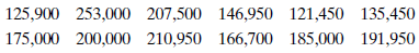
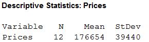
Sandy James thinks that housing prices have stabilized in the past few months. To convince her boss, she intends to compare current prices with last year's prices. She collects 12 housing prices from the want ads:
She then calculates the mean and standard deviation of the prices she has found. What are these two summary values?
She then calculates the mean and standard deviation of the prices she has found. What are these two summary values?
Question
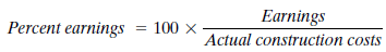
A large construction company is trying to establish a useful way to view typical profits from jobs obtained from competitive bidding. Because the jobs vary substantially in size and the final amount of the successful bid, the company has decided to express profits as percent earnings:
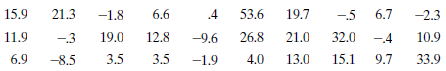
When money is lost on a project, the earnings are negative and so is the resulting net profit. A sample of 30 jobs yields these percent earnings:
a. Calculate an estimate of the mean percent earnings for the population of jobs or for all potential jobs.
b. Construct a 95% confidence interval for the mean percent earnings for the population of jobs using a large-sample argument.
c. Construct a 95% confidence interval for the mean percent earnings for the population of jobs assuming 30 is a small sample size. What additional assumption do you need to make in this case?
d. Compare the two intervals in parts b and c. Explain why a sample size of 30 is often taken as the cutoff between large and small samples.
Question
Question
Question
Question
Question
Question
Question
Population experts indicate that family size has decreased in the last few years. Ten years ago the average family size was 2.9. Consider the population of 200 family sizes given in Table P-10. Randomly select a sample of 30 family sizes and test the hypothesis that the average family size has not changed in the last 10 years.
TABLE P-10
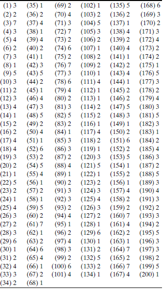
TABLE P-10
Question
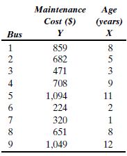
James Dobbins, maintenance supervisor for the Atlanta Transit Authority, would like to determine whether there is a positive relationship between the annual maintenance cost of a bus and its age. If a relationship exists, James feels that he can do a better job of predicting the annual bus maintenance budget. He collects the data shown in Table P-11.
a. Plot a scatter diagram.
b. What kind of relationship exists between these two variables?
c. Compute the correlation coefficient.
TABLE P-11
a. Plot a scatter diagram.
b. What kind of relationship exists between these two variables?
c. Compute the correlation coefficient.
TABLE P-11
Question
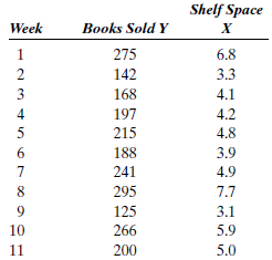
Anna Sheehan is the manager of the Spendwise supermarket chain. She would like to be able to predict paperback book sales (books per week) based on the amount of shelf display space (feet) provided. Anna gathers data for a sample of 11 weeks, as shown in Table P-12.
a. Plot a scatter diagram.
b. What kind of relationship exists between these two variables?
c. Compute the correlation coefficient. Determine the equation of the least squares line by calculating the slope and Y -intercept. Use this equation to forecast the number of books sold if 5.2 feet of shelf space is used (i.e., X = 5.2).
TABLE P-12
Question
Consider the population of 200 weekly observations presented in Table P-13. The independent variable X is the average weekly temperature of Spokane, Washington. The dependent variable Y is the number of shares of Sunshine Mining Stock traded on the Spokane exchange in a week. Randomly select data for 16 weeks and compute the coefficient of correlation. ( Hint: Make sure your sample is randomly drawn from the population.) Then determine the least squares line and forecast Y for an average weekly temperature of 63.
TABLE P-13
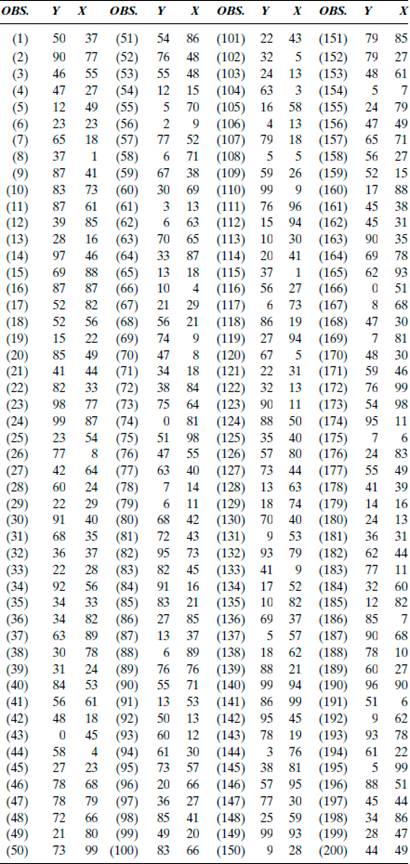
TABLE P-13
Question
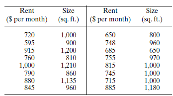
A real estate investor collects the following data on a random sample of apartments on the west side of College Station, Texas.
a. Plot the data as a scatter diagram with Y = rent and X = size.
b. Determine the equation of the fitted line relating rent to size.
c. What is the estimated increase in rent for an additional square foot of space?
d. Forecast the monthly rent for an apartment with 750 square feet.
a. Plot the data as a scatter diagram with Y = rent and X = size.
b. Determine the equation of the fitted line relating rent to size.
c. What is the estimated increase in rent for an additional square foot of space?
d. Forecast the monthly rent for an apartment with 750 square feet.
Question
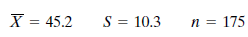
Abbott Sons needs to forecast the mean age, ? , of its hourly workforce. A random sample of personnel files is pulled with the results below. Prepare both a point estimate and a 98% confidence interval for the mean age of the entire workforce. Test the hypothesis H 0 : ? = 44 versus H 1 : ? ? 44 at the 2% level. Are the results of the hypothesis test consistent with the confidence interval for ? ? Would you expect them to be?
Question
Question
An investor with a substantial stock portfolio sued her broker and brokerage firm because lack of diversification in her portfolio led to poor performance. The rates of return for the 39 months that the account was managed by the broker produced these summary statistics:
 , S = 5.99%. Consider the 39 monthly returns as a random sample from the population of returns the brokerage would generate if it managed the account forever. Using the sample results, construct a 95% confidence interval for the mean monthly market return. Let the S P 500 represent the market, and suppose the mean S P 500 return for the same period is 0.94%. Is this a realistic value for the population mean of the client's account? Explain.
, S = 5.99%. Consider the 39 monthly returns as a random sample from the population of returns the brokerage would generate if it managed the account forever. Using the sample results, construct a 95% confidence interval for the mean monthly market return. Let the S P 500 represent the market, and suppose the mean S P 500 return for the same period is 0.94%. Is this a realistic value for the population mean of the client's account? Explain. Question
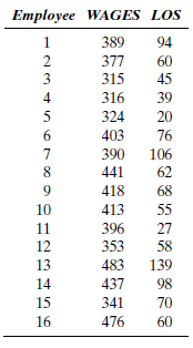
Table P-18 gives weekly wages (WAGES) in dollars and length of service (LOS) in months, at a specific point in time, for 16 women who hold customer service jobs in Texas banks.
TABLE P-18
a. Plot the data in Table P-18 as a scatter diagram with WAGES along the vertical ( Y ) axis and LOS along the horizontal ( X ) axis.
b. Calculate the sample correlation coefficient, r. Using the sign and magnitude of r , describe the nature of the linear association between WAGES and LOS. Can you think of other variables that might affect weekly wages in addition to length of service?
c. Calculate the fitted line that can be used to predict WAGES from LOS. If LOS is 80 months, what is the predicted WAGES?
Question
ALCAM ELECTRONICS
Jarrick Tilby recently received a degree in business administration from a small university and went to work for Alcam Electronics, a manufacturer of various electronic components for industry. After a few weeks on the job, he was called into the office of Alcam's owner and manager, McKennah Labrum, who asked him to investigate a question regarding a certain transistor manufactured by Alcam because a large TV company was interested in a major purchase.
McKennah wanted to forecast the average lifetime of this type of transistor, a matter of great concern to the TV company. Units currently in stock could represent those that would be produced over the lifetime of the new contract, should it be accepted.
Jarrick decided to take a random sample of the transistors in question and formulated a plan to accomplish this task. He numbered the storage bins holding the transistors, drew random bin numbers, and sampled all transistors in each selected bin for the sample. Since each bin contained about 20 transistors, he selected 10 random numbers, which gave him a final sample size of 205 transistors. Because he had selected 10 of 55 bins, he thought he had a good representative sample and could use the results of this sample to generalize to the entire population of transistors in inventory as well as to units yet to be manufactured by the same process.
Jarrick then considered the question of the average lifetime of the units. Because the unit's lifetime can extend to several years, he realized that none of the sampled units could be tested if a timely answer was desired. Therefore, he decided to contact several users of this component to determine if any lifetime records were available. Fortunately, he found three companies that had used the transistor in the past and that had limited records on component lifetimes. In total, he received data on 38 transistors whose failure times were known. Since these transistors were manufactured using the current process, he reasoned that the results of this sample could be used to make inferences about the units in inventory and those yet to be produced.
The results of the computations Jarrick performed on his sample of lifetime data follow.
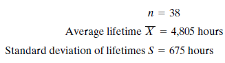
After finding that the sample average lifetime was only 4,805 hours, Jarrick was concerned because he knew the other supplier of components was guaranteeing an average lifetime of 5,000 hours. Although his sample average was a bit below 5,000 hours, he realized that the sample size was only 38 and that this did not constitute positive proof that Alcam's quality was inferior to that of the other supplier. He decided to test the hypothesis that the average lifetime of all transistors was 5,000 hours against the alternative that it was less. Following are the calculations he performed using ? =.01:

If S = 675, then the decision point is

and the decision rule is as follows:
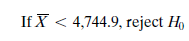
Since the sample mean (4,805) was not below the decision rule point for rejection (4,744.9), Jarrick failed to reject the hypothesis that the mean lifetime of all components was equal to 5,000 hours. He thought this would be good news to McKennah Labrum and included a summary of his findings in his final report. A few days after he gave his written and verbal report to her, McKennah called him into her office to compliment him on a good job and to share a concern she had regarding his findings. She said, "I am concerned about the very low significance level of your hypothesis test. You took only a 1% chance of rejecting the null hypothesis if it is true. This strikes me as very conservative. I am concerned that we will enter into a contract and then find that our quality level does not meet the desired 5,000-hour specification."
How would you respond to McKennah Labrum's comment?
Jarrick Tilby recently received a degree in business administration from a small university and went to work for Alcam Electronics, a manufacturer of various electronic components for industry. After a few weeks on the job, he was called into the office of Alcam's owner and manager, McKennah Labrum, who asked him to investigate a question regarding a certain transistor manufactured by Alcam because a large TV company was interested in a major purchase.
McKennah wanted to forecast the average lifetime of this type of transistor, a matter of great concern to the TV company. Units currently in stock could represent those that would be produced over the lifetime of the new contract, should it be accepted.
Jarrick decided to take a random sample of the transistors in question and formulated a plan to accomplish this task. He numbered the storage bins holding the transistors, drew random bin numbers, and sampled all transistors in each selected bin for the sample. Since each bin contained about 20 transistors, he selected 10 random numbers, which gave him a final sample size of 205 transistors. Because he had selected 10 of 55 bins, he thought he had a good representative sample and could use the results of this sample to generalize to the entire population of transistors in inventory as well as to units yet to be manufactured by the same process.
Jarrick then considered the question of the average lifetime of the units. Because the unit's lifetime can extend to several years, he realized that none of the sampled units could be tested if a timely answer was desired. Therefore, he decided to contact several users of this component to determine if any lifetime records were available. Fortunately, he found three companies that had used the transistor in the past and that had limited records on component lifetimes. In total, he received data on 38 transistors whose failure times were known. Since these transistors were manufactured using the current process, he reasoned that the results of this sample could be used to make inferences about the units in inventory and those yet to be produced.
The results of the computations Jarrick performed on his sample of lifetime data follow.
After finding that the sample average lifetime was only 4,805 hours, Jarrick was concerned because he knew the other supplier of components was guaranteeing an average lifetime of 5,000 hours. Although his sample average was a bit below 5,000 hours, he realized that the sample size was only 38 and that this did not constitute positive proof that Alcam's quality was inferior to that of the other supplier. He decided to test the hypothesis that the average lifetime of all transistors was 5,000 hours against the alternative that it was less. Following are the calculations he performed using ? =.01:
If S = 675, then the decision point is
and the decision rule is as follows:
Since the sample mean (4,805) was not below the decision rule point for rejection (4,744.9), Jarrick failed to reject the hypothesis that the mean lifetime of all components was equal to 5,000 hours. He thought this would be good news to McKennah Labrum and included a summary of his findings in his final report. A few days after he gave his written and verbal report to her, McKennah called him into her office to compliment him on a good job and to share a concern she had regarding his findings. She said, "I am concerned about the very low significance level of your hypothesis test. You took only a 1% chance of rejecting the null hypothesis if it is true. This strikes me as very conservative. I am concerned that we will enter into a contract and then find that our quality level does not meet the desired 5,000-hour specification."
How would you respond to McKennah Labrum's comment?
Question
TUX
John Mosby, owner of several Mr. Tux rental stores, is interested in forecasting his monthly sales volume (see Case 1-1). As a first step, John collects monthly sales data for the years 1998 through 2005, as shown in Table 2-10.
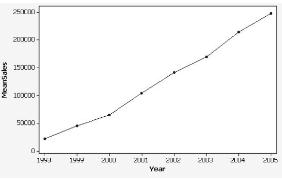
Next, John computes the average monthly sales value for each year (i.e., he adds up the 12 values for 1998 and divides by 12). John also computes the standard deviation for the 12 monthly values for each year. The results are shown in Table 2-11. John also decides to construct a time series plot, given in Figure 2-19. He plots the mean monthly sales values on the Y -axis and time on the X -axis.
TABLE 2-10 Mr. Tux Monthly Sales Data

TABLE 2-11 Mr. Tux Average Monthly Sales Values
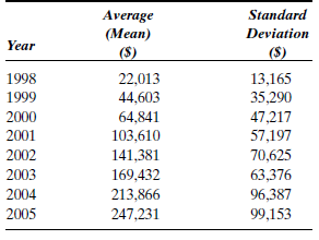
FIGURE 2-19 Mr. Tux Mean Monthly Sales
What forecasting ideas come to mind when you study John's mean monthly sales values for the years of his data?
John Mosby, owner of several Mr. Tux rental stores, is interested in forecasting his monthly sales volume (see Case 1-1). As a first step, John collects monthly sales data for the years 1998 through 2005, as shown in Table 2-10.
Next, John computes the average monthly sales value for each year (i.e., he adds up the 12 values for 1998 and divides by 12). John also computes the standard deviation for the 12 monthly values for each year. The results are shown in Table 2-11. John also decides to construct a time series plot, given in Figure 2-19. He plots the mean monthly sales values on the Y -axis and time on the X -axis.
TABLE 2-10 Mr. Tux Monthly Sales Data
TABLE 2-11 Mr. Tux Average Monthly Sales Values
FIGURE 2-19 Mr. Tux Mean Monthly Sales
What forecasting ideas come to mind when you study John's mean monthly sales values for the years of his data?
Question
TUX
John Mosby, owner of several Mr. Tux rental stores, is interested in forecasting his monthly sales volume (see Case 1-1). As a first step, John collects monthly sales data for the years 1998 through 2005, as shown in Table 2-10.
Next, John computes the average monthly sales value for each year (i.e., he adds up the 12 values for 1998 and divides by 12). John also computes the standard deviation for the 12 monthly values for each year. The results are shown in Table 2-11. John also decides to construct a time series plot, given in Figure 2-19. He plots the mean monthly sales values on the Y -axis and time on the X -axis.
TABLE 2-10 Mr. Tux Monthly Sales Data
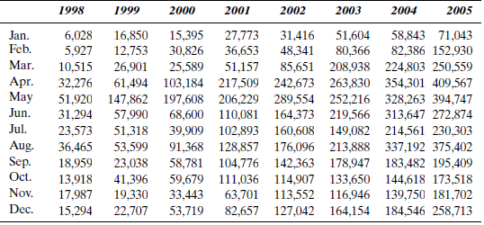
TABLE 2-11 Mr. Tux Average Monthly Sales Values

FIGURE 2-19 Mr. Tux Mean Monthly Sales

Suppose John draws a straight line freehand through his scatter diagram so that it "fits well" and then extends this line into the future, using points along the line as his monthly forecasts. How accurate do you think these forecasts will be? Use the standard deviation values John calculated in answering this question. Based on your analysis, would you encourage John to continue searching for a more accurate forecasting method? John has the latest version of Minitab on his computer. Do you think he should use the regression analysis feature of Minitab to calculate a least squares line? If he did, what X variable should he use to forecast monthly sales ( Y )?
John Mosby, owner of several Mr. Tux rental stores, is interested in forecasting his monthly sales volume (see Case 1-1). As a first step, John collects monthly sales data for the years 1998 through 2005, as shown in Table 2-10.
Next, John computes the average monthly sales value for each year (i.e., he adds up the 12 values for 1998 and divides by 12). John also computes the standard deviation for the 12 monthly values for each year. The results are shown in Table 2-11. John also decides to construct a time series plot, given in Figure 2-19. He plots the mean monthly sales values on the Y -axis and time on the X -axis.
TABLE 2-10 Mr. Tux Monthly Sales Data
TABLE 2-11 Mr. Tux Average Monthly Sales Values
FIGURE 2-19 Mr. Tux Mean Monthly Sales
Suppose John draws a straight line freehand through his scatter diagram so that it "fits well" and then extends this line into the future, using points along the line as his monthly forecasts. How accurate do you think these forecasts will be? Use the standard deviation values John calculated in answering this question. Based on your analysis, would you encourage John to continue searching for a more accurate forecasting method? John has the latest version of Minitab on his computer. Do you think he should use the regression analysis feature of Minitab to calculate a least squares line? If he did, what X variable should he use to forecast monthly sales ( Y )?
Question
ALOMEGA FOOD STORES
In Example 1.1, the president of Alomega, Julie Ruth, had collected data from her company's operations. She found several months of sales data along with several possible predictor variables (review this situation in Example 1.1). While her analysis team was working with the data in an attempt to forecast monthly sales, she became impatient and wondered which of the predictor variables was best for this purpose.
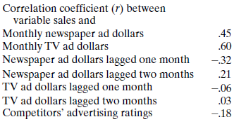
Because she had a statistical program on her desktop computer, she decided to have a look at the data herself. First, she found the correlation coefficients between the monthly sales variable and several of the potential predictor variables. Specifically, she was interested in the correlations between monthly sales and monthly newspaper ad dollars, monthly TV ad dollars, newspaper ad dollars lagged one and two months, TV ad dollars lagged one and two months, and her competitors' advertising ratings. The r values (correlation coefficients) were as follows:

Julie was not surprised to find that the highest correlation was between monthly sales and monthly TV advertising dollars ( r =.60), but she was hoping for a stronger correlation. She decided to use a regression feature to calculate the equation of the least squares line using sales as the dependent variable and monthly TV ad dollars as the predictor variable. The results of this run were
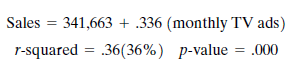
Julie had to dig out her college statistics textbook to interpret the r -squared and p -value results from her printout. After reading, she recalled that r -squared (which is the square of the correlation coefficient, r ) measures the percentage of the variability in sales that can be explained by the variability in monthly TV ad dollars (this will be explained in Chapter 6). Also, the p -value indicates that the slope coefficient (.336) is significant; that is, the hypothesis that it is zero in the population from which the sample was drawn can be rejected with almost no chance of error.
Julie concluded that the regression equation she found was significant and could be used to forecast monthly sales if the TV ad budget is known. Since TV ad expenditures are under the company's control, she felt she had a good way to forecast future sales. In a brief conversation with the head of her data management department, Roger Jackson, she mentioned her findings. He replied, "Yeah, we found that, too. But realize that TV ads explain only about a third of sales variability. OK, 36%. We really don't think that is high enough, and we're trying to use several variables together to try and get that r -squared value higher. Plus, we think we're onto a method that will do a better job than regression analysis anyway."
What do you think of Julie Ruth's analysis?
In Example 1.1, the president of Alomega, Julie Ruth, had collected data from her company's operations. She found several months of sales data along with several possible predictor variables (review this situation in Example 1.1). While her analysis team was working with the data in an attempt to forecast monthly sales, she became impatient and wondered which of the predictor variables was best for this purpose.
Because she had a statistical program on her desktop computer, she decided to have a look at the data herself. First, she found the correlation coefficients between the monthly sales variable and several of the potential predictor variables. Specifically, she was interested in the correlations between monthly sales and monthly newspaper ad dollars, monthly TV ad dollars, newspaper ad dollars lagged one and two months, TV ad dollars lagged one and two months, and her competitors' advertising ratings. The r values (correlation coefficients) were as follows:
Julie was not surprised to find that the highest correlation was between monthly sales and monthly TV advertising dollars ( r =.60), but she was hoping for a stronger correlation. She decided to use a regression feature to calculate the equation of the least squares line using sales as the dependent variable and monthly TV ad dollars as the predictor variable. The results of this run were
Julie had to dig out her college statistics textbook to interpret the r -squared and p -value results from her printout. After reading, she recalled that r -squared (which is the square of the correlation coefficient, r ) measures the percentage of the variability in sales that can be explained by the variability in monthly TV ad dollars (this will be explained in Chapter 6). Also, the p -value indicates that the slope coefficient (.336) is significant; that is, the hypothesis that it is zero in the population from which the sample was drawn can be rejected with almost no chance of error.
Julie concluded that the regression equation she found was significant and could be used to forecast monthly sales if the TV ad budget is known. Since TV ad expenditures are under the company's control, she felt she had a good way to forecast future sales. In a brief conversation with the head of her data management department, Roger Jackson, she mentioned her findings. He replied, "Yeah, we found that, too. But realize that TV ads explain only about a third of sales variability. OK, 36%. We really don't think that is high enough, and we're trying to use several variables together to try and get that r -squared value higher. Plus, we think we're onto a method that will do a better job than regression analysis anyway."
What do you think of Julie Ruth's analysis?
Question
ALOMEGA FOOD STORES
In Example 1.1, the president of Alomega, Julie Ruth, had collected data from her company's operations. She found several months of sales data along with several possible predictor variables (review this situation in Example 1.1). While her analysis team was working with the data in an attempt to forecast monthly sales, she became impatient and wondered which of the predictor variables was best for this purpose.
Because she had a statistical program on her desktop computer, she decided to have a look at the data herself. First, she found the correlation coefficients between the monthly sales variable and several of the potential predictor variables. Specifically, she was interested in the correlations between monthly sales and monthly newspaper ad dollars, monthly TV ad dollars, newspaper ad dollars lagged one and two months, TV ad dollars lagged one and two months, and her competitors' advertising ratings. The r values (correlation coefficients) were as follows:
Julie was not surprised to find that the highest correlation was between monthly sales and monthly TV advertising dollars ( r =.60), but she was hoping for a stronger correlation. She decided to use a regression feature to calculate the equation of the least squares line using sales as the dependent variable and monthly TV ad dollars as the predictor variable. The results of this run were

Julie had to dig out her college statistics textbook to interpret the r -squared and p -value results from her printout. After reading, she recalled that r -squared (which is the square of the correlation coefficient, r ) measures the percentage of the variability in sales that can be explained by the variability in monthly TV ad dollars (this will be explained in Chapter 6). Also, the p -value indicates that the slope coefficient (.336) is significant; that is, the hypothesis that it is zero in the population from which the sample was drawn can be rejected with almost no chance of error.
Julie concluded that the regression equation she found was significant and could be used to forecast monthly sales if the TV ad budget is known. Since TV ad expenditures are under the company's control, she felt she had a good way to forecast future sales. In a brief conversation with the head of her data management department, Roger Jackson, she mentioned her findings. He replied, "Yeah, we found that, too. But realize that TV ads explain only about a third of sales variability. OK, 36%. We really don't think that is high enough, and we're trying to use several variables together to try and get that r -squared value higher. Plus, we think we're onto a method that will do a better job than regression analysis anyway."
Define the residuals (errors) to be the differences between the actual sales values and the values predicted by the straight line. How might you examine the residuals to decide if Julie's straight-line representation is adequate?
In Example 1.1, the president of Alomega, Julie Ruth, had collected data from her company's operations. She found several months of sales data along with several possible predictor variables (review this situation in Example 1.1). While her analysis team was working with the data in an attempt to forecast monthly sales, she became impatient and wondered which of the predictor variables was best for this purpose.
Because she had a statistical program on her desktop computer, she decided to have a look at the data herself. First, she found the correlation coefficients between the monthly sales variable and several of the potential predictor variables. Specifically, she was interested in the correlations between monthly sales and monthly newspaper ad dollars, monthly TV ad dollars, newspaper ad dollars lagged one and two months, TV ad dollars lagged one and two months, and her competitors' advertising ratings. The r values (correlation coefficients) were as follows:
Julie was not surprised to find that the highest correlation was between monthly sales and monthly TV advertising dollars ( r =.60), but she was hoping for a stronger correlation. She decided to use a regression feature to calculate the equation of the least squares line using sales as the dependent variable and monthly TV ad dollars as the predictor variable. The results of this run were
Julie had to dig out her college statistics textbook to interpret the r -squared and p -value results from her printout. After reading, she recalled that r -squared (which is the square of the correlation coefficient, r ) measures the percentage of the variability in sales that can be explained by the variability in monthly TV ad dollars (this will be explained in Chapter 6). Also, the p -value indicates that the slope coefficient (.336) is significant; that is, the hypothesis that it is zero in the population from which the sample was drawn can be rejected with almost no chance of error.
Julie concluded that the regression equation she found was significant and could be used to forecast monthly sales if the TV ad budget is known. Since TV ad expenditures are under the company's control, she felt she had a good way to forecast future sales. In a brief conversation with the head of her data management department, Roger Jackson, she mentioned her findings. He replied, "Yeah, we found that, too. But realize that TV ads explain only about a third of sales variability. OK, 36%. We really don't think that is high enough, and we're trying to use several variables together to try and get that r -squared value higher. Plus, we think we're onto a method that will do a better job than regression analysis anyway."
Define the residuals (errors) to be the differences between the actual sales values and the values predicted by the straight line. How might you examine the residuals to decide if Julie's straight-line representation is adequate?

Unlock Deck
Sign up to unlock the cards in this deck!
Unlock Deck
Unlock Deck
1/22
Play
Full screen (f)
Deck 1: A Review of Basic Statistical Concepts
1
Sandy James thinks that housing prices have stabilized in the past few months. To convince her boss, she intends to compare current prices with last year's prices. She collects 12 housing prices from the want ads:
She then calculates the mean and standard deviation of the prices she has found. What are these two summary values?
She then calculates the mean and standard deviation of the prices she has found. What are these two summary values?
a.
Obtain the mean and standard deviation using MINITAB procedure.
MINITAB procedure:
Step 1: Choose Stat Basic Statistics Display Descriptive Statistics.
Step 2: In Variables enter the column of Prices.
Step 3: In Statistics , select Mean , StDev and N Number.
Step 4: Click OK.
MINITAB output:
 From the MINITAB output, the mean price
 is
is
 and the standard deviation
 of the prices is
 .
.
Obtain the mean and standard deviation using MINITAB procedure.
MINITAB procedure:
Step 1: Choose Stat Basic Statistics Display Descriptive Statistics.
Step 2: In Variables enter the column of Prices.
Step 3: In Statistics , select Mean , StDev and N Number.
Step 4: Click OK.
MINITAB output:
From the MINITAB output, the mean price is and the standard deviation of the prices is . 2
A large construction company is trying to establish a useful way to view typical profits from jobs obtained from competitive bidding. Because the jobs vary substantially in size and the final amount of the successful bid, the company has decided to express profits as percent earnings:
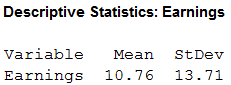
When money is lost on a project, the earnings are negative and so is the resulting net profit. A sample of 30 jobs yields these percent earnings:
a. Calculate an estimate of the mean percent earnings for the population of jobs or for all potential jobs.
b. Construct a 95% confidence interval for the mean percent earnings for the population of jobs using a large-sample argument.
c. Construct a 95% confidence interval for the mean percent earnings for the population of jobs assuming 30 is a small sample size. What additional assumption do you need to make in this case?
d. Compare the two intervals in parts b and c. Explain why a sample size of 30 is often taken as the cutoff between large and small samples.
When money is lost on a project, the earnings are negative and so is the resulting net profit. A sample of 30 jobs yields these percent earnings:
a. Calculate an estimate of the mean percent earnings for the population of jobs or for all potential jobs.
b. Construct a 95% confidence interval for the mean percent earnings for the population of jobs using a large-sample argument.
c. Construct a 95% confidence interval for the mean percent earnings for the population of jobs assuming 30 is a small sample size. What additional assumption do you need to make in this case?
d. Compare the two intervals in parts b and c. Explain why a sample size of 30 is often taken as the cutoff between large and small samples.
a.
Obtain the mean percent earnings for the population of jobs by using MINITAB.
MINITAB procedure:
Step 1: Choose Stat Basic Statistics Display Descriptive Statistics.
Step 2: In Variables , enter Earnings.
Step 3: In Statistics , select Mean and StDev.
Step 4: Click OK.
MINITAB output:
 From the above MINITAB output, the point estimate mean percent earning
 for the population of jobs is
 .
.
b.
Obtain a 95% confidence interval for the mean percent earnings for the population of jobs using a large-sample argument.
The level of significance is 0.95.
 From the table B-2, the table value of
 is given below:
 The general formula for the confidence interval estimate for population mean using large- sample argument is
 Obtain standard deviation by using MINITAB.
From the above MINITAB output in part (a), the standard deviation
 is
is
 .
.
The 95% confidence interval is obtained below:
Substitute,
 ,
,
 ,
,
 and
and
 .
.
 Therefore, the 95% confidence interval for mean percent earning for population of jobs lies between
 .
.
c.
Obtain a 95% confidence interval for the mean percent earnings for the population of jobs using a small-sample argument.
From the table B-3, the table value of
 with
with
 degrees of freedom is given below:
 Thus, the value of
 is
is
 .
.
The 95% confidence interval is obtained below:
 Thus, the 95% confidence interval for the mean percent earning for the population of jobs is
 . The additional assumption that is made in this case is that the mean percent earnings are approximately normally distributed.
d.
Explanation:
From part (b) and (c), it is clear that the confidence intervals are approximately same. This is because the multipliers 1.96 and 2.045 are almost has the same magnitude.
Obtain the mean percent earnings for the population of jobs by using MINITAB.
MINITAB procedure:
Step 1: Choose Stat Basic Statistics Display Descriptive Statistics.
Step 2: In Variables , enter Earnings.
Step 3: In Statistics , select Mean and StDev.
Step 4: Click OK.
MINITAB output:
From the above MINITAB output, the point estimate mean percent earning for the population of jobs is .b.
Obtain a 95% confidence interval for the mean percent earnings for the population of jobs using a large-sample argument.
The level of significance is 0.95.
From the table B-2, the table value of is given below: The general formula for the confidence interval estimate for population mean using large- sample argument is Obtain standard deviation by using MINITAB.From the above MINITAB output in part (a), the standard deviation
is .The 95% confidence interval is obtained below:
Substitute,
, , and . Therefore, the 95% confidence interval for mean percent earning for population of jobs lies between .c.
Obtain a 95% confidence interval for the mean percent earnings for the population of jobs using a small-sample argument.
From the table B-3, the table value of
with degrees of freedom is given below: Thus, the value of is .The 95% confidence interval is obtained below:
Thus, the 95% confidence interval for the mean percent earning for the population of jobs is . The additional assumption that is made in this case is that the mean percent earnings are approximately normally distributed.d.
Explanation:
From part (b) and (c), it is clear that the confidence intervals are approximately same. This is because the multipliers 1.96 and 2.045 are almost has the same magnitude.
3
From data on a large sample of sales transactions, a small business owner reports that a 95% confidence interval for the mean profit per transaction, ? , is (23.41, 102.59). Use these data to determine
a. A point estimate (best guess) of the mean, ? , and its 95% error margin.
b. A 90% confidence interval for the mean, ?.
a. A point estimate (best guess) of the mean, ? , and its 95% error margin.
b. A 90% confidence interval for the mean, ?.
a.
Obtain the point estimate of the mean
 .
.
The sample mean
 is the point estimate of the mean
 .
.
 Therefore, the point estimate of the mean
 is
is
 .
.
Obtain the 95% error margin.
It is given that 95% confidence interval for the mean profit per transaction is

 Therefore, the 95% error margin is
 .
.
b.
Obtain the 90% confidence interval for the mean
 .
.
For, the two-tailed test,
 From Table B-2, the required
 value for 90% confidence level is,
 Thus, the 90% confidence interval is obtained below:
 Therefore, the 90% confidence interval for the mean profit per transaction is
 .
.
Obtain the point estimate of the mean
.The sample mean
is the point estimate of the mean . Therefore, the point estimate of the mean is .Obtain the 95% error margin.
It is given that 95% confidence interval for the mean profit per transaction is
Therefore, the 95% error margin is .b.
Obtain the 90% confidence interval for the mean
.For, the two-tailed test,
From Table B-2, the required value for 90% confidence level is, Thus, the 90% confidence interval is obtained below: Therefore, the 90% confidence interval for the mean profit per transaction is . 4
We want to forecast whether the mean number of absent days per year has increased for our large workforce. A year ago the mean was known to be 12.1. A recent sample of 100 employees reveals a sample mean of 13.5 with a sample standard deviation of 1.7 days. Test at the.05 significance level to determine if the population mean has increased or if the difference between 13.5 and 12.1 simply represents sampling error.
Unlock Deck
Unlock for access to all 22 flashcards in this deck.
Unlock Deck
k this deck
5
New Horizons Airlines wants to forecast the mean number of unoccupied seats per flight to Germany next year. To develop this forecast, the records of 49 flights are randomly selected from the files for the past year, and the number of unoccupied seats is noted for each flight. The sample mean and standard deviation are 8.1 seats and 5.7 seats, respectively. Develop a point and 95% interval estimate of the mean number of unoccupied seats per flight during the past year. Forecast the mean number of unoccupied seats per flight to Germany next year. Discuss the accuracy of this forecast.
Unlock Deck
Unlock for access to all 22 flashcards in this deck.
Unlock Deck
k this deck
6
Over a period of years, a toothpaste has received a mean rating of 5.9, on a 7-point scale, for overall customer satisfaction with the product. Because of a minor unadvertised change in the product, there is concern that the customer satisfaction may have changed. Suppose the satisfaction ratings from a sample of 60 customers have a mean of 5.60 and a standard deviation of.87. Do these data indicate that the mean satisfaction rating is different from 5.9? Test with ? =.05. What is the p -value for the test?
Unlock Deck
Unlock for access to all 22 flashcards in this deck.
Unlock Deck
k this deck
7
The manager of a frozen yogurt store claims that a medium-size serving contains an average of more than 4 ounces of yogurt. From a random sample of 14 servings, she obtains a mean of 4.31 ounces and a standard deviation of.52 ounce. Test, with ? =.05, the manager's claim. Find the p -value for the test. Assume that the distribution of weight per serving is normal.
Unlock Deck
Unlock for access to all 22 flashcards in this deck.
Unlock Deck
k this deck
8
Based on past experience, the California Power Company forecasts that the mean residential electricity usage per household will be 700 kwh next January. In January, the company selects a simple random sample of 50 households and computes a mean and standard deviation of 715 and 50, respectively. Test at the.05 significance level to determine whether California Power's forecast is reasonable. Calculate and interpret the p -value for the test.
Unlock Deck
Unlock for access to all 22 flashcards in this deck.
Unlock Deck
k this deck
9
Population experts indicate that family size has decreased in the last few years. Ten years ago the average family size was 2.9. Consider the population of 200 family sizes given in Table P-10. Randomly select a sample of 30 family sizes and test the hypothesis that the average family size has not changed in the last 10 years.
TABLE P-10
TABLE P-10
Unlock Deck
Unlock for access to all 22 flashcards in this deck.
Unlock Deck
k this deck
10
James Dobbins, maintenance supervisor for the Atlanta Transit Authority, would like to determine whether there is a positive relationship between the annual maintenance cost of a bus and its age. If a relationship exists, James feels that he can do a better job of predicting the annual bus maintenance budget. He collects the data shown in Table P-11.
a. Plot a scatter diagram.
b. What kind of relationship exists between these two variables?
c. Compute the correlation coefficient.
TABLE P-11
a. Plot a scatter diagram.
b. What kind of relationship exists between these two variables?
c. Compute the correlation coefficient.
TABLE P-11
Unlock Deck
Unlock for access to all 22 flashcards in this deck.
Unlock Deck
k this deck
11
Anna Sheehan is the manager of the Spendwise supermarket chain. She would like to be able to predict paperback book sales (books per week) based on the amount of shelf display space (feet) provided. Anna gathers data for a sample of 11 weeks, as shown in Table P-12.
a. Plot a scatter diagram.
b. What kind of relationship exists between these two variables?
c. Compute the correlation coefficient. Determine the equation of the least squares line by calculating the slope and Y -intercept. Use this equation to forecast the number of books sold if 5.2 feet of shelf space is used (i.e., X = 5.2).
TABLE P-12
a. Plot a scatter diagram.
b. What kind of relationship exists between these two variables?
c. Compute the correlation coefficient. Determine the equation of the least squares line by calculating the slope and Y -intercept. Use this equation to forecast the number of books sold if 5.2 feet of shelf space is used (i.e., X = 5.2).
TABLE P-12
Unlock Deck
Unlock for access to all 22 flashcards in this deck.
Unlock Deck
k this deck
12
Consider the population of 200 weekly observations presented in Table P-13. The independent variable X is the average weekly temperature of Spokane, Washington. The dependent variable Y is the number of shares of Sunshine Mining Stock traded on the Spokane exchange in a week. Randomly select data for 16 weeks and compute the coefficient of correlation. ( Hint: Make sure your sample is randomly drawn from the population.) Then determine the least squares line and forecast Y for an average weekly temperature of 63.
TABLE P-13
TABLE P-13
Unlock Deck
Unlock for access to all 22 flashcards in this deck.
Unlock Deck
k this deck
13
A real estate investor collects the following data on a random sample of apartments on the west side of College Station, Texas.
a. Plot the data as a scatter diagram with Y = rent and X = size.
b. Determine the equation of the fitted line relating rent to size.
c. What is the estimated increase in rent for an additional square foot of space?
d. Forecast the monthly rent for an apartment with 750 square feet.
a. Plot the data as a scatter diagram with Y = rent and X = size.
b. Determine the equation of the fitted line relating rent to size.
c. What is the estimated increase in rent for an additional square foot of space?
d. Forecast the monthly rent for an apartment with 750 square feet.
Unlock Deck
Unlock for access to all 22 flashcards in this deck.
Unlock Deck
k this deck
14
Abbott Sons needs to forecast the mean age, ? , of its hourly workforce. A random sample of personnel files is pulled with the results below. Prepare both a point estimate and a 98% confidence interval for the mean age of the entire workforce. Test the hypothesis H 0 : ? = 44 versus H 1 : ? ? 44 at the 2% level. Are the results of the hypothesis test consistent with the confidence interval for ? ? Would you expect them to be?
Unlock Deck
Unlock for access to all 22 flashcards in this deck.
Unlock Deck
k this deck
15
In each of the following situations, state an appropriate null hypothesis, H 0 , and alternative hypothesis, H 1. Identify the parameter that you use to state the hypotheses.
a. Census Bureau data show that the mean household income in the area served by a shopping mall is $63,700 per year. A market research firm surveys shoppers at the mall to find out whether the mean household income of mall shoppers is higher than that of the general population.
b. Last year the local fire department took an average of 4.3 minutes to respond to calls. Do this year's data show a different average response time?
c. The mean area of several thousand apartments in a new development is advertised to be 1,300 square feet. A tenant group thinks that the apartments are smaller than advertised. They hire an engineer to measure a sample of apartments to test their suspicion.
Unlock Deck
Unlock for access to all 22 flashcards in this deck.
Unlock Deck
k this deck
16
An investor with a substantial stock portfolio sued her broker and brokerage firm because lack of diversification in her portfolio led to poor performance. The rates of return for the 39 months that the account was managed by the broker produced these summary statistics:
, S = 5.99%. Consider the 39 monthly returns as a random sample from the population of returns the brokerage would generate if it managed the account forever. Using the sample results, construct a 95% confidence interval for the mean monthly market return. Let the S P 500 represent the market, and suppose the mean S P 500 return for the same period is 0.94%. Is this a realistic value for the population mean of the client's account? Explain.
, S = 5.99%. Consider the 39 monthly returns as a random sample from the population of returns the brokerage would generate if it managed the account forever. Using the sample results, construct a 95% confidence interval for the mean monthly market return. Let the S P 500 represent the market, and suppose the mean S P 500 return for the same period is 0.94%. Is this a realistic value for the population mean of the client's account? Explain. Unlock Deck
Unlock for access to all 22 flashcards in this deck.
Unlock Deck
k this deck
17
Table P-18 gives weekly wages (WAGES) in dollars and length of service (LOS) in months, at a specific point in time, for 16 women who hold customer service jobs in Texas banks.
TABLE P-18
a. Plot the data in Table P-18 as a scatter diagram with WAGES along the vertical ( Y ) axis and LOS along the horizontal ( X ) axis.
b. Calculate the sample correlation coefficient, r. Using the sign and magnitude of r , describe the nature of the linear association between WAGES and LOS. Can you think of other variables that might affect weekly wages in addition to length of service?
c. Calculate the fitted line that can be used to predict WAGES from LOS. If LOS is 80 months, what is the predicted WAGES?
TABLE P-18
a. Plot the data in Table P-18 as a scatter diagram with WAGES along the vertical ( Y ) axis and LOS along the horizontal ( X ) axis.
b. Calculate the sample correlation coefficient, r. Using the sign and magnitude of r , describe the nature of the linear association between WAGES and LOS. Can you think of other variables that might affect weekly wages in addition to length of service?
c. Calculate the fitted line that can be used to predict WAGES from LOS. If LOS is 80 months, what is the predicted WAGES?
Unlock Deck
Unlock for access to all 22 flashcards in this deck.
Unlock Deck
k this deck
18
ALCAM ELECTRONICS
Jarrick Tilby recently received a degree in business administration from a small university and went to work for Alcam Electronics, a manufacturer of various electronic components for industry. After a few weeks on the job, he was called into the office of Alcam's owner and manager, McKennah Labrum, who asked him to investigate a question regarding a certain transistor manufactured by Alcam because a large TV company was interested in a major purchase.
McKennah wanted to forecast the average lifetime of this type of transistor, a matter of great concern to the TV company. Units currently in stock could represent those that would be produced over the lifetime of the new contract, should it be accepted.
Jarrick decided to take a random sample of the transistors in question and formulated a plan to accomplish this task. He numbered the storage bins holding the transistors, drew random bin numbers, and sampled all transistors in each selected bin for the sample. Since each bin contained about 20 transistors, he selected 10 random numbers, which gave him a final sample size of 205 transistors. Because he had selected 10 of 55 bins, he thought he had a good representative sample and could use the results of this sample to generalize to the entire population of transistors in inventory as well as to units yet to be manufactured by the same process.
Jarrick then considered the question of the average lifetime of the units. Because the unit's lifetime can extend to several years, he realized that none of the sampled units could be tested if a timely answer was desired. Therefore, he decided to contact several users of this component to determine if any lifetime records were available. Fortunately, he found three companies that had used the transistor in the past and that had limited records on component lifetimes. In total, he received data on 38 transistors whose failure times were known. Since these transistors were manufactured using the current process, he reasoned that the results of this sample could be used to make inferences about the units in inventory and those yet to be produced.
The results of the computations Jarrick performed on his sample of lifetime data follow.
After finding that the sample average lifetime was only 4,805 hours, Jarrick was concerned because he knew the other supplier of components was guaranteeing an average lifetime of 5,000 hours. Although his sample average was a bit below 5,000 hours, he realized that the sample size was only 38 and that this did not constitute positive proof that Alcam's quality was inferior to that of the other supplier. He decided to test the hypothesis that the average lifetime of all transistors was 5,000 hours against the alternative that it was less. Following are the calculations he performed using ? =.01:
If S = 675, then the decision point is
and the decision rule is as follows:
Since the sample mean (4,805) was not below the decision rule point for rejection (4,744.9), Jarrick failed to reject the hypothesis that the mean lifetime of all components was equal to 5,000 hours. He thought this would be good news to McKennah Labrum and included a summary of his findings in his final report. A few days after he gave his written and verbal report to her, McKennah called him into her office to compliment him on a good job and to share a concern she had regarding his findings. She said, "I am concerned about the very low significance level of your hypothesis test. You took only a 1% chance of rejecting the null hypothesis if it is true. This strikes me as very conservative. I am concerned that we will enter into a contract and then find that our quality level does not meet the desired 5,000-hour specification."
How would you respond to McKennah Labrum's comment?
Unlock Deck
Unlock for access to all 22 flashcards in this deck.
Unlock Deck
k this deck
19
TUX
John Mosby, owner of several Mr. Tux rental stores, is interested in forecasting his monthly sales volume (see Case 1-1). As a first step, John collects monthly sales data for the years 1998 through 2005, as shown in Table 2-10.
Next, John computes the average monthly sales value for each year (i.e., he adds up the 12 values for 1998 and divides by 12). John also computes the standard deviation for the 12 monthly values for each year. The results are shown in Table 2-11. John also decides to construct a time series plot, given in Figure 2-19. He plots the mean monthly sales values on the Y -axis and time on the X -axis.
TABLE 2-10 Mr. Tux Monthly Sales Data
TABLE 2-11 Mr. Tux Average Monthly Sales Values
FIGURE 2-19 Mr. Tux Mean Monthly Sales
What forecasting ideas come to mind when you study John's mean monthly sales values for the years of his data?
Unlock Deck
Unlock for access to all 22 flashcards in this deck.
Unlock Deck
k this deck
20
TUX
John Mosby, owner of several Mr. Tux rental stores, is interested in forecasting his monthly sales volume (see Case 1-1). As a first step, John collects monthly sales data for the years 1998 through 2005, as shown in Table 2-10.
Next, John computes the average monthly sales value for each year (i.e., he adds up the 12 values for 1998 and divides by 12). John also computes the standard deviation for the 12 monthly values for each year. The results are shown in Table 2-11. John also decides to construct a time series plot, given in Figure 2-19. He plots the mean monthly sales values on the Y -axis and time on the X -axis.
TABLE 2-10 Mr. Tux Monthly Sales Data
TABLE 2-11 Mr. Tux Average Monthly Sales Values
FIGURE 2-19 Mr. Tux Mean Monthly Sales
Suppose John draws a straight line freehand through his scatter diagram so that it "fits well" and then extends this line into the future, using points along the line as his monthly forecasts. How accurate do you think these forecasts will be? Use the standard deviation values John calculated in answering this question. Based on your analysis, would you encourage John to continue searching for a more accurate forecasting method? John has the latest version of Minitab on his computer. Do you think he should use the regression analysis feature of Minitab to calculate a least squares line? If he did, what X variable should he use to forecast monthly sales ( Y )?
Unlock Deck
Unlock for access to all 22 flashcards in this deck.
Unlock Deck
k this deck
21
ALOMEGA FOOD STORES
In Example 1.1, the president of Alomega, Julie Ruth, had collected data from her company's operations. She found several months of sales data along with several possible predictor variables (review this situation in Example 1.1). While her analysis team was working with the data in an attempt to forecast monthly sales, she became impatient and wondered which of the predictor variables was best for this purpose.
Because she had a statistical program on her desktop computer, she decided to have a look at the data herself. First, she found the correlation coefficients between the monthly sales variable and several of the potential predictor variables. Specifically, she was interested in the correlations between monthly sales and monthly newspaper ad dollars, monthly TV ad dollars, newspaper ad dollars lagged one and two months, TV ad dollars lagged one and two months, and her competitors' advertising ratings. The r values (correlation coefficients) were as follows:
Julie was not surprised to find that the highest correlation was between monthly sales and monthly TV advertising dollars ( r =.60), but she was hoping for a stronger correlation. She decided to use a regression feature to calculate the equation of the least squares line using sales as the dependent variable and monthly TV ad dollars as the predictor variable. The results of this run were
Julie had to dig out her college statistics textbook to interpret the r -squared and p -value results from her printout. After reading, she recalled that r -squared (which is the square of the correlation coefficient, r ) measures the percentage of the variability in sales that can be explained by the variability in monthly TV ad dollars (this will be explained in Chapter 6). Also, the p -value indicates that the slope coefficient (.336) is significant; that is, the hypothesis that it is zero in the population from which the sample was drawn can be rejected with almost no chance of error.
Julie concluded that the regression equation she found was significant and could be used to forecast monthly sales if the TV ad budget is known. Since TV ad expenditures are under the company's control, she felt she had a good way to forecast future sales. In a brief conversation with the head of her data management department, Roger Jackson, she mentioned her findings. He replied, "Yeah, we found that, too. But realize that TV ads explain only about a third of sales variability. OK, 36%. We really don't think that is high enough, and we're trying to use several variables together to try and get that r -squared value higher. Plus, we think we're onto a method that will do a better job than regression analysis anyway."
What do you think of Julie Ruth's analysis?
Unlock Deck
Unlock for access to all 22 flashcards in this deck.
Unlock Deck
k this deck
22
ALOMEGA FOOD STORES
In Example 1.1, the president of Alomega, Julie Ruth, had collected data from her company's operations. She found several months of sales data along with several possible predictor variables (review this situation in Example 1.1). While her analysis team was working with the data in an attempt to forecast monthly sales, she became impatient and wondered which of the predictor variables was best for this purpose.
Because she had a statistical program on her desktop computer, she decided to have a look at the data herself. First, she found the correlation coefficients between the monthly sales variable and several of the potential predictor variables. Specifically, she was interested in the correlations between monthly sales and monthly newspaper ad dollars, monthly TV ad dollars, newspaper ad dollars lagged one and two months, TV ad dollars lagged one and two months, and her competitors' advertising ratings. The r values (correlation coefficients) were as follows:
Julie was not surprised to find that the highest correlation was between monthly sales and monthly TV advertising dollars ( r =.60), but she was hoping for a stronger correlation. She decided to use a regression feature to calculate the equation of the least squares line using sales as the dependent variable and monthly TV ad dollars as the predictor variable. The results of this run were
Julie had to dig out her college statistics textbook to interpret the r -squared and p -value results from her printout. After reading, she recalled that r -squared (which is the square of the correlation coefficient, r ) measures the percentage of the variability in sales that can be explained by the variability in monthly TV ad dollars (this will be explained in Chapter 6). Also, the p -value indicates that the slope coefficient (.336) is significant; that is, the hypothesis that it is zero in the population from which the sample was drawn can be rejected with almost no chance of error.
Julie concluded that the regression equation she found was significant and could be used to forecast monthly sales if the TV ad budget is known. Since TV ad expenditures are under the company's control, she felt she had a good way to forecast future sales. In a brief conversation with the head of her data management department, Roger Jackson, she mentioned her findings. He replied, "Yeah, we found that, too. But realize that TV ads explain only about a third of sales variability. OK, 36%. We really don't think that is high enough, and we're trying to use several variables together to try and get that r -squared value higher. Plus, we think we're onto a method that will do a better job than regression analysis anyway."
Define the residuals (errors) to be the differences between the actual sales values and the values predicted by the straight line. How might you examine the residuals to decide if Julie's straight-line representation is adequate?
Unlock Deck
Unlock for access to all 22 flashcards in this deck.
Unlock Deck
k this deck
Unlock Deck
Unlock for access to all 22 flashcards in this deck.


