Deck 15: Multiple Regression Model Building
Full screen (f)
Question
Which of the following is used to find a "best" model?
A)Odds ratio
B)Mallow's
C)Standard error of the estimate
D)SST
A)Odds ratio
B)Mallow's
C)Standard error of the estimate
D)SST
Question
SCENARIO 15-2 In Hawaii, condemnation proceedings are under way to enable private citizens to own the property that their homes are built on.Until recently, only estates were permitted to own land, and homeowners leased the land from the estate.In order to comply with the new law, a large Hawaiian estate wants to use regression analysis to estimate the fair market value of the land. The following model was fit to data collected for n = 20 properties, 10 of which are located near a cove. Model 1:  where Y
  Sale price of property in thousands of dollars
  Size of property in thousands of square feet
  1 if property located near cove, 0 if not Using the data collected for the 20 properties, the following partial output obtained from Microsoft Excel is shown: SUMMARY OUTPUT
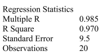

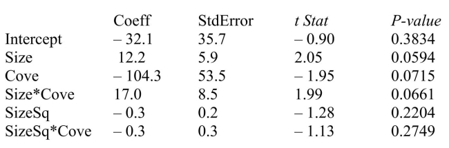
Referring to Scenario 15-2, given a quadratic relationship between sale price (Y)and property size , what test should be used to test whether the curves differ from cove and non-cove properties?
A)F test for the entire regression model.
B)t test on each of the coefficients in the entire regression model.
C)Partial F test on the subset of the appropriate coefficients.
D)t test on each of the subsets of the appropriate coefficients.
where Y Sale price of property in thousands of dollars Size of property in thousands of square feet 1 if property located near cove, 0 if not Using the data collected for the 20 properties, the following partial output obtained from Microsoft Excel is shown: SUMMARY OUTPUT Referring to Scenario 15-2, given a quadratic relationship between sale price (Y)and property size
, what test should be used to test whether the curves differ from cove and non-cove properties?A)F test for the entire regression model.
B)t test on each of the coefficients in the entire regression model.
C)Partial F test on the subset of the appropriate coefficients.
D)t test on each of the subsets of the appropriate coefficients.
Question
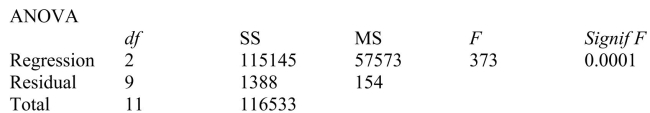
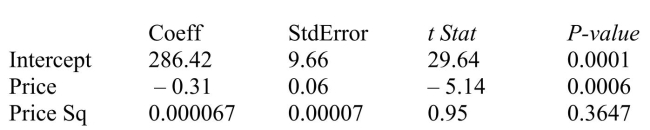
SCENARIO 15-1 A certain type of rare gem serves as a status symbol for many of its owners.In theory, for low prices, the demand increases, and it decreases as the price of the gem increases.However, experts hypothesize that when the gem is valued at very high prices, the demand increases with price due to the status owners believe they gain in obtaining the gem.Thus, the model proposed to best explain the demand for the gem by its price is the quadratic model: 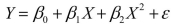 where Y = demand (in thousands)and X = retail price per carat. This model was fit to data collected for a sample of 12 rare gems of this type.A portion of the computer analysis obtained from Microsoft Excel is shown below: SUMMARY OUTPUT
Referring to Scenario 15-1, does there appear to be significant upward curvature in the response curve relating the demand (Y)and the price (X)at 10% level of significance?
A)Yes, since the p-value for the test is less than 0.10.
B)No, since the value of is near 0.
C)No, since the p-value for the test is greater than 0.10.
D)Yes, since the value of is positive.
where Y = demand (in thousands)and X = retail price per carat. This model was fit to data collected for a sample of 12 rare gems of this type.A portion of the computer analysis obtained from Microsoft Excel is shown below: SUMMARY OUTPUT Referring to Scenario 15-1, does there appear to be significant upward curvature in the response curve relating the demand (Y)and the price (X)at 10% level of significance?
A)Yes, since the p-value for the test is less than 0.10.
B)No, since the value of
is near 0.C)No, since the p-value for the test is greater than 0.10.
D)Yes, since the value of
is positive. Question
SCENARIO 15-2 In Hawaii, condemnation proceedings are under way to enable private citizens to own the property that their homes are built on.Until recently, only estates were permitted to own land, and homeowners leased the land from the estate.In order to comply with the new law, a large Hawaiian estate wants to use regression analysis to estimate the fair market value of the land. The following model was fit to data collected for n = 20 properties, 10 of which are located near a cove. Model 1: where Y Sale price of property in thousands of dollars Size of property in thousands of square feet 1 if property located near cove, 0 if not Using the data collected for the 20 properties, the following partial output obtained from Microsoft Excel is shown: SUMMARY OUTPUT
Referring to Scenario 15-2, is the overall model statistically adequate at a 0.05 level of significance for predicting sale price (Y)?
A)No, since some of the t tests for the individual variables are not significant.
B)No, since the standard deviation of the model is fairly large.
C)Yes, since none of the estimates are equal to 0.
D)Yes, since the significance of the F-value for the test is smaller than 0.05.
where Y Sale price of property in thousands of dollars Size of property in thousands of square feet 1 if property located near cove, 0 if not Using the data collected for the 20 properties, the following partial output obtained from Microsoft Excel is shown: SUMMARY OUTPUT Referring to Scenario 15-2, is the overall model statistically adequate at a 0.05 level of significance for predicting sale price (Y)?
A)No, since some of the t tests for the individual variables are not significant.
B)No, since the standard deviation of the model is fairly large.
C)Yes, since none of the
estimates are equal to 0.D)Yes, since the significance of the F-value for the test is smaller than 0.05.
Question
Question
SCENARIO 15-1 A certain type of rare gem serves as a status symbol for many of its owners.In theory, for low prices, the demand increases, and it decreases as the price of the gem increases.However, experts hypothesize that when the gem is valued at very high prices, the demand increases with price due to the status owners believe they gain in obtaining the gem.Thus, the model proposed to best explain the demand for the gem by its price is the quadratic model: where Y = demand (in thousands)and X = retail price per carat. This model was fit to data collected for a sample of 12 rare gems of this type.A portion of the computer analysis obtained from Microsoft Excel is shown below: SUMMARY OUTPUT
Referring to Scenario 15-1, a more parsimonious simple linear model is likely to be statistically superior to the fitted curvilinear for predicting sale price (Y).
where Y = demand (in thousands)and X = retail price per carat. This model was fit to data collected for a sample of 12 rare gems of this type.A portion of the computer analysis obtained from Microsoft Excel is shown below: SUMMARY OUTPUT Referring to Scenario 15-1, a more parsimonious simple linear model is likely to be statistically superior to the fitted curvilinear for predicting sale price (Y).
Question
SCENARIO 15-1 A certain type of rare gem serves as a status symbol for many of its owners.In theory, for low prices, the demand increases, and it decreases as the price of the gem increases.However, experts hypothesize that when the gem is valued at very high prices, the demand increases with price due to the status owners believe they gain in obtaining the gem.Thus, the model proposed to best explain the demand for the gem by its price is the quadratic model: where Y = demand (in thousands)and X = retail price per carat. This model was fit to data collected for a sample of 12 rare gems of this type.A portion of the computer analysis obtained from Microsoft Excel is shown below: SUMMARY OUTPUT
Referring to Scenario 15-1, what is the correct interpretation of the coefficient of multiple determination?
A)98.8% of the total variation in demand can be explained by the linear relationship between demand and price.
B)98.8% of the total variation in demand can be explained by the quadratic relationship between demand and price.
C)98.8% of the total variation in demand can be explained by the addition of the square term in price.
D)98.8% of the total variation in demand can be explained by just the square term in price.
where Y = demand (in thousands)and X = retail price per carat. This model was fit to data collected for a sample of 12 rare gems of this type.A portion of the computer analysis obtained from Microsoft Excel is shown below: SUMMARY OUTPUT Referring to Scenario 15-1, what is the correct interpretation of the coefficient of multiple determination?
A)98.8% of the total variation in demand can be explained by the linear relationship between demand and price.
B)98.8% of the total variation in demand can be explained by the quadratic relationship between demand and price.
C)98.8% of the total variation in demand can be explained by the addition of the square term in price.
D)98.8% of the total variation in demand can be explained by just the square term in price.
Question
Question
Question
As a project for his business statistics class, a student examined the factors that determined parking meter rates throughout the campus area.Data were collected for the price per hour of parking, blocks to the quadrangle, and one of the three jurisdictions: on campus, in downtown and off campus, or outside of downtown and off campus.The population regression model hypothesized is 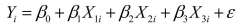 where Y is the meter price
  is the number of blocks to the quad
  is a dummy variable that takes the value 1 if the meter is located in downtown and off campus and the value 0 otherwise
  is a dummy variable that takes the value 1 if the meter is located outside of downtown and off campus, and the value 0 otherwise Suppose that whether the meter is located on campus is an important explanatory factor. Why should the variable that depicts this attribute not be included in the model?
A)Its inclusion will introduce autocorrelation.
B)Its inclusion will introduce collinearity.
C)Its inclusion will inflate the standard errors of the estimated coefficients.
D)Both (b)and (c).
where Y is the meter price is the number of blocks to the quad is a dummy variable that takes the value 1 if the meter is located in downtown and off campus and the value 0 otherwise is a dummy variable that takes the value 1 if the meter is located outside of downtown and off campus, and the value 0 otherwise Suppose that whether the meter is located on campus is an important explanatory factor. Why should the variable that depicts this attribute not be included in the model?A)Its inclusion will introduce autocorrelation.
B)Its inclusion will introduce collinearity.
C)Its inclusion will inflate the standard errors of the estimated coefficients.
D)Both (b)and (c).
Question
The  statistic is used
A)to determine if there is a problem of collinearity.
B)if the variances of the error terms are all the same in a regression model.
C)to choose the best model.
D)to determine if there is an irregular component in a time series.
statistic is usedA)to determine if there is a problem of collinearity.
B)if the variances of the error terms are all the same in a regression model.
C)to choose the best model.
D)to determine if there is an irregular component in a time series.
Question
Question
SCENARIO 15-2 In Hawaii, condemnation proceedings are under way to enable private citizens to own the property that their homes are built on.Until recently, only estates were permitted to own land, and homeowners leased the land from the estate.In order to comply with the new law, a large Hawaiian estate wants to use regression analysis to estimate the fair market value of the land. The following model was fit to data collected for n = 20 properties, 10 of which are located near a cove. Model 1: where Y Sale price of property in thousands of dollars Size of property in thousands of square feet 1 if property located near cove, 0 if not Using the data collected for the 20 properties, the following partial output obtained from Microsoft Excel is shown: SUMMARY OUTPUT
Referring to Scenario 15-2, given a quadratic relationship between sale price (Y)and property size , what null hypothesis would you test to determine whether the curves differ from cove and non-cove properties?
A)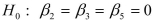
B)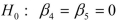
C)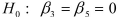
D)
where Y Sale price of property in thousands of dollars Size of property in thousands of square feet 1 if property located near cove, 0 if not Using the data collected for the 20 properties, the following partial output obtained from Microsoft Excel is shown: SUMMARY OUTPUT Referring to Scenario 15-2, given a quadratic relationship between sale price (Y)and property size
, what null hypothesis would you test to determine whether the curves differ from cove and non-cove properties?A)
B)
C)
D)
Question
Question
SCENARIO 15-1 A certain type of rare gem serves as a status symbol for many of its owners.In theory, for low prices, the demand increases, and it decreases as the price of the gem increases.However, experts hypothesize that when the gem is valued at very high prices, the demand increases with price due to the status owners believe they gain in obtaining the gem.Thus, the model proposed to best explain the demand for the gem by its price is the quadratic model: where Y = demand (in thousands)and X = retail price per carat. This model was fit to data collected for a sample of 12 rare gems of this type.A portion of the computer analysis obtained from Microsoft Excel is shown below: SUMMARY OUTPUT
Referring to Scenario 15-1, what is the p-value associated with the test statistic for testing whether there is an upward curvature in the response curve relating the demand (Y)and the price (X)?
A)0.0001
B)0.0006
C)0.3647
D)None of the above.
where Y = demand (in thousands)and X = retail price per carat. This model was fit to data collected for a sample of 12 rare gems of this type.A portion of the computer analysis obtained from Microsoft Excel is shown below: SUMMARY OUTPUT Referring to Scenario 15-1, what is the p-value associated with the test statistic for testing whether there is an upward curvature in the response curve relating the demand (Y)and the price (X)?
A)0.0001
B)0.0006
C)0.3647
D)None of the above.
Question
Question
Question
SCENARIO 15-1 A certain type of rare gem serves as a status symbol for many of its owners.In theory, for low prices, the demand increases, and it decreases as the price of the gem increases.However, experts hypothesize that when the gem is valued at very high prices, the demand increases with price due to the status owners believe they gain in obtaining the gem.Thus, the model proposed to best explain the demand for the gem by its price is the quadratic model: where Y = demand (in thousands)and X = retail price per carat. This model was fit to data collected for a sample of 12 rare gems of this type.A portion of the computer analysis obtained from Microsoft Excel is shown below: SUMMARY OUTPUT
Referring to Scenario 15-1, what is the value of the test statistic for testing whether there is an upward curvature in the response curve relating the demand (Y)and the price (X)?
A)-5.14
B)0.95
C)373
D)None of the above.
where Y = demand (in thousands)and X = retail price per carat. This model was fit to data collected for a sample of 12 rare gems of this type.A portion of the computer analysis obtained from Microsoft Excel is shown below: SUMMARY OUTPUT Referring to Scenario 15-1, what is the value of the test statistic for testing whether there is an upward curvature in the response curve relating the demand (Y)and the price (X)?
A)-5.14
B)0.95
C)373
D)None of the above.
Question
Question
Question
Question
SCENARIO 15-3 A chemist employed by a pharmaceutical firm has developed a muscle relaxant.She took a sample of 14 people suffering from extreme muscle constriction.She gave each a vial containing a dose (X)of the drug and recorded the time to relief (Y)measured in seconds for each.She fit a curvilinear model to this data.The results obtained by Microsoft Excel follow SUMMARY OUTPUT 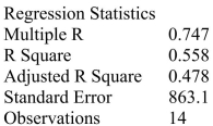
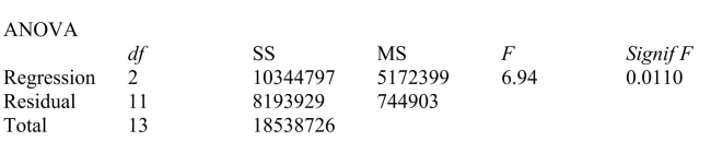
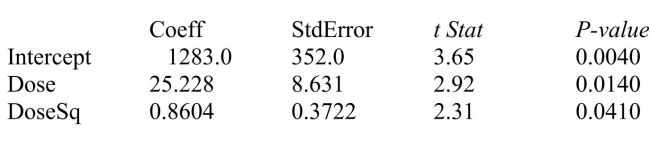
Referring to Scenario 15-3, suppose the chemist decides to use an F test to determine if there is a significant curvilinear relationship between time and dose.The p-value of the test is ________.
Referring to Scenario 15-3, suppose the chemist decides to use an F test to determine if there is a significant curvilinear relationship between time and dose.The p-value of the test is ________.
Question
Question
Question
Question
SCENARIO 15-3 A chemist employed by a pharmaceutical firm has developed a muscle relaxant.She took a sample of 14 people suffering from extreme muscle constriction.She gave each a vial containing a dose (X)of the drug and recorded the time to relief (Y)measured in seconds for each.She fit a curvilinear model to this data.The results obtained by Microsoft Excel follow SUMMARY OUTPUT
Referring to Scenario 15-3, the prediction of time to relief for a person receiving a dose of 10 units of the drug is ________.
Referring to Scenario 15-3, the prediction of time to relief for a person receiving a dose of 10 units of the drug is ________.
Question
SCENARIO 15-3 A chemist employed by a pharmaceutical firm has developed a muscle relaxant.She took a sample of 14 people suffering from extreme muscle constriction.She gave each a vial containing a dose (X)of the drug and recorded the time to relief (Y)measured in seconds for each.She fit a curvilinear model to this data.The results obtained by Microsoft Excel follow SUMMARY OUTPUT
Referring to Scenario 15-3, suppose the chemist decides to use an F test to determine if there is a significant curvilinear relationship between time and dose.If she chooses to use a level of significance of 0.05, she would decide that there is a significant curvilinear relationship.
Referring to Scenario 15-3, suppose the chemist decides to use an F test to determine if there is a significant curvilinear relationship between time and dose.If she chooses to use a level of significance of 0.05, she would decide that there is a significant curvilinear relationship.
Question
SCENARIO 15-3 A chemist employed by a pharmaceutical firm has developed a muscle relaxant.She took a sample of 14 people suffering from extreme muscle constriction.She gave each a vial containing a dose (X)of the drug and recorded the time to relief (Y)measured in seconds for each.She fit a curvilinear model to this data.The results obtained by Microsoft Excel follow SUMMARY OUTPUT
Referring to Scenario 15-3, suppose the chemist decides to use a t test to determine if there is a significant difference between a linear model and a curvilinear model that includes a linear term.If she used a level of significance of 0.05, she would decide that the linear model is sufficient.
Referring to Scenario 15-3, suppose the chemist decides to use a t test to determine if there is a significant difference between a linear model and a curvilinear model that includes a linear term.If she used a level of significance of 0.05, she would decide that the linear model is sufficient.
Question
SCENARIO 15-3 A chemist employed by a pharmaceutical firm has developed a muscle relaxant.She took a sample of 14 people suffering from extreme muscle constriction.She gave each a vial containing a dose (X)of the drug and recorded the time to relief (Y)measured in seconds for each.She fit a curvilinear model to this data.The results obtained by Microsoft Excel follow SUMMARY OUTPUT
Referring to Scenario 15-3, suppose the chemist decides to use a t test to determine if the linear term is significant.The value of the test statistic is ______.
Referring to Scenario 15-3, suppose the chemist decides to use a t test to determine if the linear term is significant.The value of the test statistic is ______.
Question
SCENARIO 15-3 A chemist employed by a pharmaceutical firm has developed a muscle relaxant.She took a sample of 14 people suffering from extreme muscle constriction.She gave each a vial containing a dose (X)of the drug and recorded the time to relief (Y)measured in seconds for each.She fit a curvilinear model to this data.The results obtained by Microsoft Excel follow SUMMARY OUTPUT
Referring to Scenario 15-3, suppose the chemist decides to use an F test to determine if there is a significant curvilinear relationship between time and dose.If she chooses to use a level of significance of 0.01 she would decide that there is a significant curvilinear relationship.
Referring to Scenario 15-3, suppose the chemist decides to use an F test to determine if there is a significant curvilinear relationship between time and dose.If she chooses to use a level of significance of 0.01 she would decide that there is a significant curvilinear relationship.
Question
SCENARIO 15-3 A chemist employed by a pharmaceutical firm has developed a muscle relaxant.She took a sample of 14 people suffering from extreme muscle constriction.She gave each a vial containing a dose (X)of the drug and recorded the time to relief (Y)measured in seconds for each.She fit a curvilinear model to this data.The results obtained by Microsoft Excel follow SUMMARY OUTPUT
Referring to Scenario 15-3, suppose the chemist decides to use an F test to determine if there is a significant curvilinear relationship between time and dose.The value of the test statistic is ________.
Referring to Scenario 15-3, suppose the chemist decides to use an F test to determine if there is a significant curvilinear relationship between time and dose.The value of the test statistic is ________.
Question
Question
SCENARIO 15-3 A chemist employed by a pharmaceutical firm has developed a muscle relaxant.She took a sample of 14 people suffering from extreme muscle constriction.She gave each a vial containing a dose (X)of the drug and recorded the time to relief (Y)measured in seconds for each.She fit a curvilinear model to this data.The results obtained by Microsoft Excel follow SUMMARY OUTPUT
Referring to Scenario 15-3, suppose the chemist decides to use a t test to determine if there is a significant difference between a linear model and a curvilinear model that includes a linear term.The p-value of the test statistic for the contribution of the curvilinear term is ________.
Referring to Scenario 15-3, suppose the chemist decides to use a t test to determine if there is a significant difference between a linear model and a curvilinear model that includes a linear term.The p-value of the test statistic for the contribution of the curvilinear term is ________.
Question
SCENARIO 15-3 A chemist employed by a pharmaceutical firm has developed a muscle relaxant.She took a sample of 14 people suffering from extreme muscle constriction.She gave each a vial containing a dose (X)of the drug and recorded the time to relief (Y)measured in seconds for each.She fit a curvilinear model to this data.The results obtained by Microsoft Excel follow SUMMARY OUTPUT
Referring to Scenario 15-3, suppose the chemist decides to use a t test to determine if the linear term is significant.Using a level of significance of 0.05, she would decide that the linear term is significant.
Referring to Scenario 15-3, suppose the chemist decides to use a t test to determine if the linear term is significant.Using a level of significance of 0.05, she would decide that the linear term is significant.
Question
Two simple regression models were used to predict a single dependent variable.Both models were highly significant, but when the two independent variables were placed in the same multiple regression model for the dependent variable,  did not increase substantially and the parameter estimates for the model were not significantly different from 0.This is probably an example of collinearity.
did not increase substantially and the parameter estimates for the model were not significantly different from 0.This is probably an example of collinearity. Question
SCENARIO 15-3 A chemist employed by a pharmaceutical firm has developed a muscle relaxant.She took a sample of 14 people suffering from extreme muscle constriction.She gave each a vial containing a dose (X)of the drug and recorded the time to relief (Y)measured in seconds for each.She fit a curvilinear model to this data.The results obtained by Microsoft Excel follow SUMMARY OUTPUT
Referring to Scenario 15-3, suppose the chemist decides to use a t test to determine if the linear term is significant.The p-value of the test is ______.
Referring to Scenario 15-3, suppose the chemist decides to use a t test to determine if the linear term is significant.The p-value of the test is ______.
Question
A high value of  significantly above 0 in multiple regression accompanied by insignificant t-values on all parameter estimates very often indicates a high correlation between independent variables in the model.
significantly above 0 in multiple regression accompanied by insignificant t-values on all parameter estimates very often indicates a high correlation between independent variables in the model. Question
Question
SCENARIO 15-3 A chemist employed by a pharmaceutical firm has developed a muscle relaxant.She took a sample of 14 people suffering from extreme muscle constriction.She gave each a vial containing a dose (X)of the drug and recorded the time to relief (Y)measured in seconds for each.She fit a curvilinear model to this data.The results obtained by Microsoft Excel follow SUMMARY OUTPUT
Referring to Scenario 15-3, suppose the chemist decides to use a t test to determine if there is a significant difference between a linear model and a curvilinear model that includes a linear term.If she used a level of significance of 0.01, she would decide that the linear model is sufficient.
Referring to Scenario 15-3, suppose the chemist decides to use a t test to determine if there is a significant difference between a linear model and a curvilinear model that includes a linear term.If she used a level of significance of 0.01, she would decide that the linear model is sufficient.
Question
Question
Question
Question
SCENARIO 15-4 The superintendent of a school district wanted to predict the percentage of students passing a sixth-grade proficiency test.She obtained the data on percentage of students passing the proficiency test (% Passing), daily mean of the percentage of students attending class (% Attendance), mean teacher salary in dollars (Salaries), and instructional spending per pupil in dollars (Spending)of 47 schools in the state. Let Y = % Passing as the dependent variable,  Attendance,
  Salaries and
  Spending. The coefficient of multiple determination (
  )of each of the 3 predictors with all the other remaining predictors are, respectively, 0.0338, 0.4669, and 0.4743. The output from the best-subset regressions is given below:
 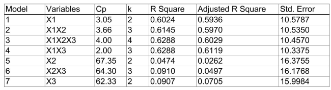 Following is the residual plot for % Attendance:
 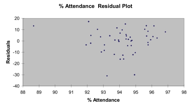 Following is the output of several multiple regression models:
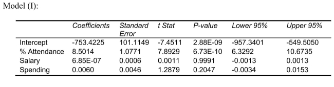
Referring to Scenario 15-4, which of the following models should be taken into consideration using the Mallows' statistic?
A)
B)
C)both of the above
D)None of the above
Attendance, Salaries and Spending. The coefficient of multiple determination ( )of each of the 3 predictors with all the other remaining predictors are, respectively, 0.0338, 0.4669, and 0.4743. The output from the best-subset regressions is given below: Following is the residual plot for % Attendance: Following is the output of several multiple regression models: Referring to Scenario 15-4, which of the following models should be taken into consideration using the Mallows'
statistic?A)
B)
C)both of the above
D)None of the above
Question
Using the best-subsets approach to model building, models are being considered when their
A)
B)
C)
D)
A)
B)
C)
D)
Question
SCENARIO 15-4 The superintendent of a school district wanted to predict the percentage of students passing a sixth-grade proficiency test.She obtained the data on percentage of students passing the proficiency test (% Passing), daily mean of the percentage of students attending class (% Attendance), mean teacher salary in dollars (Salaries), and instructional spending per pupil in dollars (Spending)of 47 schools in the state. Let Y = % Passing as the dependent variable, Attendance, Salaries and Spending. The coefficient of multiple determination ( )of each of the 3 predictors with all the other remaining predictors are, respectively, 0.0338, 0.4669, and 0.4743. The output from the best-subset regressions is given below: Following is the residual plot for % Attendance: Following is the output of several multiple regression models:
Referring to Scenario 15-4, the better model using a 5% level of significance derived from the "best" model above is
A)
B)
C)
D)
Attendance, Salaries and Spending. The coefficient of multiple determination ( )of each of the 3 predictors with all the other remaining predictors are, respectively, 0.0338, 0.4669, and 0.4743. The output from the best-subset regressions is given below: Following is the residual plot for % Attendance: Following is the output of several multiple regression models: Referring to Scenario 15-4, the better model using a 5% level of significance derived from the "best" model above is
A)
B)
C)
D)
Question
SCENARIO 15-4 The superintendent of a school district wanted to predict the percentage of students passing a sixth-grade proficiency test.She obtained the data on percentage of students passing the proficiency test (% Passing), daily mean of the percentage of students attending class (% Attendance), mean teacher salary in dollars (Salaries), and instructional spending per pupil in dollars (Spending)of 47 schools in the state. Let Y = % Passing as the dependent variable, Attendance, Salaries and Spending. The coefficient of multiple determination ( )of each of the 3 predictors with all the other remaining predictors are, respectively, 0.0338, 0.4669, and 0.4743. The output from the best-subset regressions is given below: Following is the residual plot for % Attendance: Following is the output of several multiple regression models:
Referring to Scenario 15-4, there is reason to suspect collinearity between some pairs of predictors.
Attendance, Salaries and Spending. The coefficient of multiple determination ( )of each of the 3 predictors with all the other remaining predictors are, respectively, 0.0338, 0.4669, and 0.4743. The output from the best-subset regressions is given below: Following is the residual plot for % Attendance: Following is the output of several multiple regression models: Referring to Scenario 15-4, there is reason to suspect collinearity between some pairs of predictors.
Question
Using the Cp statistic in model building, all models with  are equally good.
are equally good. Question
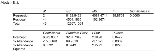
An independent variable  is considered highly correlated with the other independent variables if
A)
B)
C)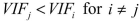
D)
is considered highly correlated with the other independent variables ifA)
B)
C)
D)
Question
SCENARIO 15-4 The superintendent of a school district wanted to predict the percentage of students passing a sixth-grade proficiency test.She obtained the data on percentage of students passing the proficiency test (% Passing), daily mean of the percentage of students attending class (% Attendance), mean teacher salary in dollars (Salaries), and instructional spending per pupil in dollars (Spending)of 47 schools in the state. Let Y = % Passing as the dependent variable, Attendance, Salaries and Spending. The coefficient of multiple determination ( )of each of the 3 predictors with all the other remaining predictors are, respectively, 0.0338, 0.4669, and 0.4743. The output from the best-subset regressions is given below: Following is the residual plot for % Attendance: Following is the output of several multiple regression models:
Referring to Scenario 15-4, which of the following predictors should first be dropped to remove collinearity?
A)
B)
C)
D)None of the above
Attendance, Salaries and Spending. The coefficient of multiple determination ( )of each of the 3 predictors with all the other remaining predictors are, respectively, 0.0338, 0.4669, and 0.4743. The output from the best-subset regressions is given below: Following is the residual plot for % Attendance: Following is the output of several multiple regression models: Referring to Scenario 15-4, which of the following predictors should first be dropped to remove collinearity?
A)
B)
C)
D)None of the above
Question
Question
Question
Question
SCENARIO 15-4 The superintendent of a school district wanted to predict the percentage of students passing a sixth-grade proficiency test.She obtained the data on percentage of students passing the proficiency test (% Passing), daily mean of the percentage of students attending class (% Attendance), mean teacher salary in dollars (Salaries), and instructional spending per pupil in dollars (Spending)of 47 schools in the state. Let Y = % Passing as the dependent variable, Attendance, Salaries and Spending. The coefficient of multiple determination ( )of each of the 3 predictors with all the other remaining predictors are, respectively, 0.0338, 0.4669, and 0.4743. The output from the best-subset regressions is given below: Following is the residual plot for % Attendance: Following is the output of several multiple regression models:
Referring to Scenario 15-4, the "best" model using a 5% level of significance among those chosen by the statistic is
A)
B)
C)either of the above
D)None of the above
Attendance, Salaries and Spending. The coefficient of multiple determination ( )of each of the 3 predictors with all the other remaining predictors are, respectively, 0.0338, 0.4669, and 0.4743. The output from the best-subset regressions is given below: Following is the residual plot for % Attendance: Following is the output of several multiple regression models: Referring to Scenario 15-4, the "best" model using a 5% level of significance among those chosen by the
statistic isA)
B)
C)either of the above
D)None of the above
Question
SCENARIO 15-4 The superintendent of a school district wanted to predict the percentage of students passing a sixth-grade proficiency test.She obtained the data on percentage of students passing the proficiency test (% Passing), daily mean of the percentage of students attending class (% Attendance), mean teacher salary in dollars (Salaries), and instructional spending per pupil in dollars (Spending)of 47 schools in the state. Let Y = % Passing as the dependent variable, Attendance, Salaries and Spending. The coefficient of multiple determination ( )of each of the 3 predictors with all the other remaining predictors are, respectively, 0.0338, 0.4669, and 0.4743. The output from the best-subset regressions is given below: Following is the residual plot for % Attendance: Following is the output of several multiple regression models:
Referring to Scenario 15-4, what are, respectively, the values of the variance inflationary factor of the 3 predictors?
Attendance, Salaries and Spending. The coefficient of multiple determination ( )of each of the 3 predictors with all the other remaining predictors are, respectively, 0.0338, 0.4669, and 0.4743. The output from the best-subset regressions is given below: Following is the residual plot for % Attendance: Following is the output of several multiple regression models: Referring to Scenario 15-4, what are, respectively, the values of the variance inflationary factor of the 3 predictors?
Question
Question
Question
Question
SCENARIO 15-4 The superintendent of a school district wanted to predict the percentage of students passing a sixth-grade proficiency test.She obtained the data on percentage of students passing the proficiency test (% Passing), daily mean of the percentage of students attending class (% Attendance), mean teacher salary in dollars (Salaries), and instructional spending per pupil in dollars (Spending)of 47 schools in the state. Let Y = % Passing as the dependent variable, Attendance, Salaries and Spending. The coefficient of multiple determination ( )of each of the 3 predictors with all the other remaining predictors are, respectively, 0.0338, 0.4669, and 0.4743. The output from the best-subset regressions is given below: Following is the residual plot for % Attendance: Following is the output of several multiple regression models:
Referring to Scenario 15-4, the residual plot suggests that a nonlinear model on % attendance may be a better model.
Attendance, Salaries and Spending. The coefficient of multiple determination ( )of each of the 3 predictors with all the other remaining predictors are, respectively, 0.0338, 0.4669, and 0.4743. The output from the best-subset regressions is given below: Following is the residual plot for % Attendance: Following is the output of several multiple regression models: Referring to Scenario 15-4, the residual plot suggests that a nonlinear model on % attendance may be a better model.
Question
Question
SCENARIO 15-4 The superintendent of a school district wanted to predict the percentage of students passing a sixth-grade proficiency test.She obtained the data on percentage of students passing the proficiency test (% Passing), daily mean of the percentage of students attending class (% Attendance), mean teacher salary in dollars (Salaries), and instructional spending per pupil in dollars (Spending)of 47 schools in the state. Let Y = % Passing as the dependent variable, Attendance, Salaries and Spending. The coefficient of multiple determination ( )of each of the 3 predictors with all the other remaining predictors are, respectively, 0.0338, 0.4669, and 0.4743. The output from the best-subset regressions is given below: Following is the residual plot for % Attendance: Following is the output of several multiple regression models:
Referring to Scenario 15-4, the "best" model chosen using the adjusted R-square statistic is
A)
B)
C)either of the above
D)None of the above
Attendance, Salaries and Spending. The coefficient of multiple determination ( )of each of the 3 predictors with all the other remaining predictors are, respectively, 0.0338, 0.4669, and 0.4743. The output from the best-subset regressions is given below: Following is the residual plot for % Attendance: Following is the output of several multiple regression models: Referring to Scenario 15-4, the "best" model chosen using the adjusted R-square statistic is
A)
B)
C)either of the above
D)None of the above
Question
SCENARIO 15-4 The superintendent of a school district wanted to predict the percentage of students passing a sixth-grade proficiency test.She obtained the data on percentage of students passing the proficiency test (% Passing), daily mean of the percentage of students attending class (% Attendance), mean teacher salary in dollars (Salaries), and instructional spending per pupil in dollars (Spending)of 47 schools in the state. Let Y = % Passing as the dependent variable, Attendance, Salaries and Spending. The coefficient of multiple determination ( )of each of the 3 predictors with all the other remaining predictors are, respectively, 0.0338, 0.4669, and 0.4743. The output from the best-subset regressions is given below: Following is the residual plot for % Attendance: Following is the output of several multiple regression models:
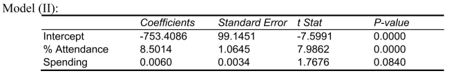
what is the p-value of the test statistic to determine whether the quadratic effect of daily average of the percentage of students attending class on percentage of students passing the proficiency test is significant at a 5% level of significance?
Attendance, Salaries and Spending. The coefficient of multiple determination ( )of each of the 3 predictors with all the other remaining predictors are, respectively, 0.0338, 0.4669, and 0.4743. The output from the best-subset regressions is given below: Following is the residual plot for % Attendance: Following is the output of several multiple regression models: what is the p-value of the test statistic to determine whether the quadratic effect of daily average of the percentage of students attending class on percentage of students passing the proficiency test is significant at a 5% level of significance?
Question
SCENARIO 15-6 Given below are results from the regression analysis on 40 observations where the dependent variable is the number of weeks a worker is unemployed due to a layoff (Y)and the independent variables are the age of the worker (  ), the number of years of education received (
  ), the number of years at the previous job (
  ), a dummy variable for marital status (
  1 = married, 0 = otherwise), a dummy variable for head of household (
  1 = yes, 0 = no)and a dummy variable for management position (
  1 = yes, 0 = no). The coefficient of multiple determination (
  )for the regression model using each of the 6 variables
  as the dependent variable and all other X variables as independent variables are, respectively, 0.2628, 0.1240, 0.2404, 0.3510, 0.3342 and 0.0993. The partial results from best-subset regression are given below:
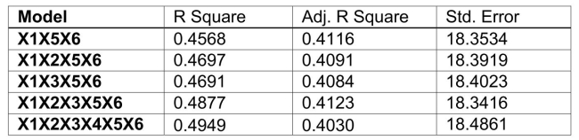
Referring to Scenario 15-6, what is the value of the variance inflationary factor of Head?
), the number of years of education received ( ), the number of years at the previous job ( ), a dummy variable for marital status ( 1 = married, 0 = otherwise), a dummy variable for head of household ( 1 = yes, 0 = no)and a dummy variable for management position ( 1 = yes, 0 = no). The coefficient of multiple determination ( )for the regression model using each of the 6 variables as the dependent variable and all other X variables as independent variables are, respectively, 0.2628, 0.1240, 0.2404, 0.3510, 0.3342 and 0.0993. The partial results from best-subset regression are given below: Referring to Scenario 15-6, what is the value of the variance inflationary factor of Head?
Question
SCENARIO 15-6 Given below are results from the regression analysis on 40 observations where the dependent variable is the number of weeks a worker is unemployed due to a layoff (Y)and the independent variables are the age of the worker ( ), the number of years of education received ( ), the number of years at the previous job ( ), a dummy variable for marital status ( 1 = married, 0 = otherwise), a dummy variable for head of household ( 1 = yes, 0 = no)and a dummy variable for management position ( 1 = yes, 0 = no). The coefficient of multiple determination ( )for the regression model using each of the 6 variables as the dependent variable and all other X variables as independent variables are, respectively, 0.2628, 0.1240, 0.2404, 0.3510, 0.3342 and 0.0993. The partial results from best-subset regression are given below:
Referring to Scenario 15-6, the variable X3 should be dropped to remove collinearity?
), the number of years of education received ( ), the number of years at the previous job ( ), a dummy variable for marital status ( 1 = married, 0 = otherwise), a dummy variable for head of household ( 1 = yes, 0 = no)and a dummy variable for management position ( 1 = yes, 0 = no). The coefficient of multiple determination ( )for the regression model using each of the 6 variables as the dependent variable and all other X variables as independent variables are, respectively, 0.2628, 0.1240, 0.2404, 0.3510, 0.3342 and 0.0993. The partial results from best-subset regression are given below: Referring to Scenario 15-6, the variable X3 should be dropped to remove collinearity?
Question
SCENARIO 15-6 Given below are results from the regression analysis on 40 observations where the dependent variable is the number of weeks a worker is unemployed due to a layoff (Y)and the independent variables are the age of the worker ( ), the number of years of education received ( ), the number of years at the previous job ( ), a dummy variable for marital status ( 1 = married, 0 = otherwise), a dummy variable for head of household ( 1 = yes, 0 = no)and a dummy variable for management position ( 1 = yes, 0 = no). The coefficient of multiple determination ( )for the regression model using each of the 6 variables as the dependent variable and all other X variables as independent variables are, respectively, 0.2628, 0.1240, 0.2404, 0.3510, 0.3342 and 0.0993. The partial results from best-subset regression are given below:
Referring to Scenario 15-6, what is the value of the variance inflationary factor of Edu?
), the number of years of education received ( ), the number of years at the previous job ( ), a dummy variable for marital status ( 1 = married, 0 = otherwise), a dummy variable for head of household ( 1 = yes, 0 = no)and a dummy variable for management position ( 1 = yes, 0 = no). The coefficient of multiple determination ( )for the regression model using each of the 6 variables as the dependent variable and all other X variables as independent variables are, respectively, 0.2628, 0.1240, 0.2404, 0.3510, 0.3342 and 0.0993. The partial results from best-subset regression are given below: Referring to Scenario 15-6, what is the value of the variance inflationary factor of Edu?
Question
SCENARIO 15-4 The superintendent of a school district wanted to predict the percentage of students passing a sixth-grade proficiency test.She obtained the data on percentage of students passing the proficiency test (% Passing), daily mean of the percentage of students attending class (% Attendance), mean teacher salary in dollars (Salaries), and instructional spending per pupil in dollars (Spending)of 47 schools in the state. Let Y = % Passing as the dependent variable, Attendance, Salaries and Spending. The coefficient of multiple determination ( )of each of the 3 predictors with all the other remaining predictors are, respectively, 0.0338, 0.4669, and 0.4743. The output from the best-subset regressions is given below: Following is the residual plot for % Attendance: Following is the output of several multiple regression models:
Referring to Scenario 15-4, The superintendent wants to know the quadratic effect of average percentage of students attending class on the percentage of students passing the proficiency test.What is the value of the test statistic?
Attendance, Salaries and Spending. The coefficient of multiple determination ( )of each of the 3 predictors with all the other remaining predictors are, respectively, 0.0338, 0.4669, and 0.4743. The output from the best-subset regressions is given below: Following is the residual plot for % Attendance: Following is the output of several multiple regression models: Referring to Scenario 15-4, The superintendent wants to know the quadratic effect of average percentage of students attending class on the percentage of students passing the proficiency test.What is the value of the test statistic?
Question
SCENARIO 15-6 Given below are results from the regression analysis on 40 observations where the dependent variable is the number of weeks a worker is unemployed due to a layoff (Y)and the independent variables are the age of the worker ( ), the number of years of education received ( ), the number of years at the previous job ( ), a dummy variable for marital status ( 1 = married, 0 = otherwise), a dummy variable for head of household ( 1 = yes, 0 = no)and a dummy variable for management position ( 1 = yes, 0 = no). The coefficient of multiple determination ( )for the regression model using each of the 6 variables as the dependent variable and all other X variables as independent variables are, respectively, 0.2628, 0.1240, 0.2404, 0.3510, 0.3342 and 0.0993. The partial results from best-subset regression are given below:
Referring to Scenario 15-6, the variable x₁ should be dropped to remove collinearity?
), the number of years of education received ( ), the number of years at the previous job ( ), a dummy variable for marital status ( 1 = married, 0 = otherwise), a dummy variable for head of household ( 1 = yes, 0 = no)and a dummy variable for management position ( 1 = yes, 0 = no). The coefficient of multiple determination ( )for the regression model using each of the 6 variables as the dependent variable and all other X variables as independent variables are, respectively, 0.2628, 0.1240, 0.2404, 0.3510, 0.3342 and 0.0993. The partial results from best-subset regression are given below: Referring to Scenario 15-6, the variable x₁ should be dropped to remove collinearity?
Question
SCENARIO 15-6 Given below are results from the regression analysis on 40 observations where the dependent variable is the number of weeks a worker is unemployed due to a layoff (Y)and the independent variables are the age of the worker ( ), the number of years of education received ( ), the number of years at the previous job ( ), a dummy variable for marital status ( 1 = married, 0 = otherwise), a dummy variable for head of household ( 1 = yes, 0 = no)and a dummy variable for management position ( 1 = yes, 0 = no). The coefficient of multiple determination ( )for the regression model using each of the 6 variables as the dependent variable and all other X variables as independent variables are, respectively, 0.2628, 0.1240, 0.2404, 0.3510, 0.3342 and 0.0993. The partial results from best-subset regression are given below:
Referring to Scenario 15-6, the variable x₂ should be dropped to remove collinearity?
), the number of years of education received ( ), the number of years at the previous job ( ), a dummy variable for marital status ( 1 = married, 0 = otherwise), a dummy variable for head of household ( 1 = yes, 0 = no)and a dummy variable for management position ( 1 = yes, 0 = no). The coefficient of multiple determination ( )for the regression model using each of the 6 variables as the dependent variable and all other X variables as independent variables are, respectively, 0.2628, 0.1240, 0.2404, 0.3510, 0.3342 and 0.0993. The partial results from best-subset regression are given below: Referring to Scenario 15-6, the variable x₂ should be dropped to remove collinearity?
Question
SCENARIO 15-5 What are the factors that determine the acceleration time (in sec.)from 0 to 60 miles per hour of a car? Data on the following variables for 171 different vehicle models were collected: Accel Time: Acceleration time in sec. Cargo Vol: Cargo volume in cu.ft. HP: Horsepower MPG: Miles per gallon SUV: 1 if the vehicle model is an SUV with Coupe as the base when SUV and Sedan are both 0 Sedan: 1 if the vehicle model is a sedan with Coupe as the base when SUV and Sedan are both 0 The coefficient of multiple determination (  )for the regression model using each of the 5 variables
  as the dependent variable and all other X variables as independent variables are, respectively, 0.7461, 0.5676, 0.6764, 0.8582, 0.6632.
Referring to Scenario 15-5, what is the value of the variance inflationary factor of
)for the regression model using each of the 5 variables as the dependent variable and all other X variables as independent variables are, respectively, 0.7461, 0.5676, 0.6764, 0.8582, 0.6632.Referring to Scenario 15-5, what is the value of the variance inflationary factor of
Question
SCENARIO 15-5 What are the factors that determine the acceleration time (in sec.)from 0 to 60 miles per hour of a car? Data on the following variables for 171 different vehicle models were collected: Accel Time: Acceleration time in sec. Cargo Vol: Cargo volume in cu.ft. HP: Horsepower MPG: Miles per gallon SUV: 1 if the vehicle model is an SUV with Coupe as the base when SUV and Sedan are both 0 Sedan: 1 if the vehicle model is a sedan with Coupe as the base when SUV and Sedan are both 0 The coefficient of multiple determination ( )for the regression model using each of the 5 variables as the dependent variable and all other X variables as independent variables are, respectively, 0.7461, 0.5676, 0.6764, 0.8582, 0.6632.
Referring to Scenario 15-5, there is reason to suspect collinearity between some pairs of predictors based on the values of the variance inflationary factor.
)for the regression model using each of the 5 variables as the dependent variable and all other X variables as independent variables are, respectively, 0.7461, 0.5676, 0.6764, 0.8582, 0.6632.Referring to Scenario 15-5, there is reason to suspect collinearity between some pairs of predictors based on the values of the variance inflationary factor.
Question
SCENARIO 15-6 Given below are results from the regression analysis on 40 observations where the dependent variable is the number of weeks a worker is unemployed due to a layoff (Y)and the independent variables are the age of the worker ( ), the number of years of education received ( ), the number of years at the previous job ( ), a dummy variable for marital status ( 1 = married, 0 = otherwise), a dummy variable for head of household ( 1 = yes, 0 = no)and a dummy variable for management position ( 1 = yes, 0 = no). The coefficient of multiple determination ( )for the regression model using each of the 6 variables as the dependent variable and all other X variables as independent variables are, respectively, 0.2628, 0.1240, 0.2404, 0.3510, 0.3342 and 0.0993. The partial results from best-subset regression are given below:
Referring to Scenario 15-6, what is the value of the variance inflationary factor of Manager?
), the number of years of education received ( ), the number of years at the previous job ( ), a dummy variable for marital status ( 1 = married, 0 = otherwise), a dummy variable for head of household ( 1 = yes, 0 = no)and a dummy variable for management position ( 1 = yes, 0 = no). The coefficient of multiple determination ( )for the regression model using each of the 6 variables as the dependent variable and all other X variables as independent variables are, respectively, 0.2628, 0.1240, 0.2404, 0.3510, 0.3342 and 0.0993. The partial results from best-subset regression are given below: Referring to Scenario 15-6, what is the value of the variance inflationary factor of Manager?
Question
SCENARIO 15-5 What are the factors that determine the acceleration time (in sec.)from 0 to 60 miles per hour of a car? Data on the following variables for 171 different vehicle models were collected: Accel Time: Acceleration time in sec. Cargo Vol: Cargo volume in cu.ft. HP: Horsepower MPG: Miles per gallon SUV: 1 if the vehicle model is an SUV with Coupe as the base when SUV and Sedan are both 0 Sedan: 1 if the vehicle model is a sedan with Coupe as the base when SUV and Sedan are both 0 The coefficient of multiple determination ( )for the regression model using each of the 5 variables as the dependent variable and all other X variables as independent variables are, respectively, 0.7461, 0.5676, 0.6764, 0.8582, 0.6632.
Referring to Scenario 15-5, what is the value of the variance inflationary factor of Sedan?
)for the regression model using each of the 5 variables as the dependent variable and all other X variables as independent variables are, respectively, 0.7461, 0.5676, 0.6764, 0.8582, 0.6632.Referring to Scenario 15-5, what is the value of the variance inflationary factor of Sedan?
Question
SCENARIO 15-4 The superintendent of a school district wanted to predict the percentage of students passing a sixth-grade proficiency test.She obtained the data on percentage of students passing the proficiency test (% Passing), daily mean of the percentage of students attending class (% Attendance), mean teacher salary in dollars (Salaries), and instructional spending per pupil in dollars (Spending)of 47 schools in the state. Let Y = % Passing as the dependent variable, Attendance, Salaries and Spending. The coefficient of multiple determination ( )of each of the 3 predictors with all the other remaining predictors are, respectively, 0.0338, 0.4669, and 0.4743. The output from the best-subset regressions is given below: Following is the residual plot for % Attendance: Following is the output of several multiple regression models:
Referring to Scenario 15-4, the null hypothesis should be rejected when testing whether the quadratic effect of daily average of the percentage of students attending class on percentage of students passing the proficiency test is significant at a 5% level of significance.
Attendance, Salaries and Spending. The coefficient of multiple determination ( )of each of the 3 predictors with all the other remaining predictors are, respectively, 0.0338, 0.4669, and 0.4743. The output from the best-subset regressions is given below: Following is the residual plot for % Attendance: Following is the output of several multiple regression models: Referring to Scenario 15-4, the null hypothesis should be rejected when testing whether the quadratic effect of daily average of the percentage of students attending class on percentage of students passing the proficiency test is significant at a 5% level of significance.
Question
SCENARIO 15-5 What are the factors that determine the acceleration time (in sec.)from 0 to 60 miles per hour of a car? Data on the following variables for 171 different vehicle models were collected: Accel Time: Acceleration time in sec. Cargo Vol: Cargo volume in cu.ft. HP: Horsepower MPG: Miles per gallon SUV: 1 if the vehicle model is an SUV with Coupe as the base when SUV and Sedan are both 0 Sedan: 1 if the vehicle model is a sedan with Coupe as the base when SUV and Sedan are both 0 The coefficient of multiple determination ( )for the regression model using each of the 5 variables as the dependent variable and all other X variables as independent variables are, respectively, 0.7461, 0.5676, 0.6764, 0.8582, 0.6632.
Referring to Scenario 15-5, what is the value of the variance inflationary factor of Cargo Vol?
)for the regression model using each of the 5 variables as the dependent variable and all other X variables as independent variables are, respectively, 0.7461, 0.5676, 0.6764, 0.8582, 0.6632.Referring to Scenario 15-5, what is the value of the variance inflationary factor of Cargo Vol?
Question
SCENARIO 15-5 What are the factors that determine the acceleration time (in sec.)from 0 to 60 miles per hour of a car? Data on the following variables for 171 different vehicle models were collected: Accel Time: Acceleration time in sec. Cargo Vol: Cargo volume in cu.ft. HP: Horsepower MPG: Miles per gallon SUV: 1 if the vehicle model is an SUV with Coupe as the base when SUV and Sedan are both 0 Sedan: 1 if the vehicle model is a sedan with Coupe as the base when SUV and Sedan are both 0 The coefficient of multiple determination ( )for the regression model using each of the 5 variables as the dependent variable and all other X variables as independent variables are, respectively, 0.7461, 0.5676, 0.6764, 0.8582, 0.6632.
Referring to Scenario 15-5, what is the value of the variance inflationary factor of SUV?
)for the regression model using each of the 5 variables as the dependent variable and all other X variables as independent variables are, respectively, 0.7461, 0.5676, 0.6764, 0.8582, 0.6632.Referring to Scenario 15-5, what is the value of the variance inflationary factor of SUV?
Question
SCENARIO 15-4 The superintendent of a school district wanted to predict the percentage of students passing a sixth-grade proficiency test.She obtained the data on percentage of students passing the proficiency test (% Passing), daily mean of the percentage of students attending class (% Attendance), mean teacher salary in dollars (Salaries), and instructional spending per pupil in dollars (Spending)of 47 schools in the state. Let Y = % Passing as the dependent variable, Attendance, Salaries and Spending. The coefficient of multiple determination ( )of each of the 3 predictors with all the other remaining predictors are, respectively, 0.0338, 0.4669, and 0.4743. The output from the best-subset regressions is given below: Following is the residual plot for % Attendance: Following is the output of several multiple regression models:
Referring to Scenario 15-4, the quadratic effect of daily average of the percentage of students attending class on percentage of students passing the proficiency test is not significant at a 5% level of significance.
Attendance, Salaries and Spending. The coefficient of multiple determination ( )of each of the 3 predictors with all the other remaining predictors are, respectively, 0.0338, 0.4669, and 0.4743. The output from the best-subset regressions is given below: Following is the residual plot for % Attendance: Following is the output of several multiple regression models: Referring to Scenario 15-4, the quadratic effect of daily average of the percentage of students attending class on percentage of students passing the proficiency test is not significant at a 5% level of significance.
Question
SCENARIO 15-6 Given below are results from the regression analysis on 40 observations where the dependent variable is the number of weeks a worker is unemployed due to a layoff (Y)and the independent variables are the age of the worker ( ), the number of years of education received ( ), the number of years at the previous job ( ), a dummy variable for marital status ( 1 = married, 0 = otherwise), a dummy variable for head of household ( 1 = yes, 0 = no)and a dummy variable for management position ( 1 = yes, 0 = no). The coefficient of multiple determination ( )for the regression model using each of the 6 variables as the dependent variable and all other X variables as independent variables are, respectively, 0.2628, 0.1240, 0.2404, 0.3510, 0.3342 and 0.0993. The partial results from best-subset regression are given below:
Referring to Scenario 15-6, what is the value of the variance inflationary factor of Married?
), the number of years of education received ( ), the number of years at the previous job ( ), a dummy variable for marital status ( 1 = married, 0 = otherwise), a dummy variable for head of household ( 1 = yes, 0 = no)and a dummy variable for management position ( 1 = yes, 0 = no). The coefficient of multiple determination ( )for the regression model using each of the 6 variables as the dependent variable and all other X variables as independent variables are, respectively, 0.2628, 0.1240, 0.2404, 0.3510, 0.3342 and 0.0993. The partial results from best-subset regression are given below: Referring to Scenario 15-6, what is the value of the variance inflationary factor of Married?
Question
SCENARIO 15-5 What are the factors that determine the acceleration time (in sec.)from 0 to 60 miles per hour of a car? Data on the following variables for 171 different vehicle models were collected: Accel Time: Acceleration time in sec. Cargo Vol: Cargo volume in cu.ft. HP: Horsepower MPG: Miles per gallon SUV: 1 if the vehicle model is an SUV with Coupe as the base when SUV and Sedan are both 0 Sedan: 1 if the vehicle model is a sedan with Coupe as the base when SUV and Sedan are both 0 The coefficient of multiple determination ( )for the regression model using each of the 5 variables as the dependent variable and all other X variables as independent variables are, respectively, 0.7461, 0.5676, 0.6764, 0.8582, 0.6632.
Referring to Scenario 15-5, what is the value of the variance inflationary factor of HP?
)for the regression model using each of the 5 variables as the dependent variable and all other X variables as independent variables are, respectively, 0.7461, 0.5676, 0.6764, 0.8582, 0.6632.Referring to Scenario 15-5, what is the value of the variance inflationary factor of HP?
Question
SCENARIO 15-6 Given below are results from the regression analysis on 40 observations where the dependent variable is the number of weeks a worker is unemployed due to a layoff (Y)and the independent variables are the age of the worker ( ), the number of years of education received ( ), the number of years at the previous job ( ), a dummy variable for marital status ( 1 = married, 0 = otherwise), a dummy variable for head of household ( 1 = yes, 0 = no)and a dummy variable for management position ( 1 = yes, 0 = no). The coefficient of multiple determination ( )for the regression model using each of the 6 variables as the dependent variable and all other X variables as independent variables are, respectively, 0.2628, 0.1240, 0.2404, 0.3510, 0.3342 and 0.0993. The partial results from best-subset regression are given below:
Referring to Scenario 15-6, what is the value of the variance inflationary factor of Job Yr?
), the number of years of education received ( ), the number of years at the previous job ( ), a dummy variable for marital status ( 1 = married, 0 = otherwise), a dummy variable for head of household ( 1 = yes, 0 = no)and a dummy variable for management position ( 1 = yes, 0 = no). The coefficient of multiple determination ( )for the regression model using each of the 6 variables as the dependent variable and all other X variables as independent variables are, respectively, 0.2628, 0.1240, 0.2404, 0.3510, 0.3342 and 0.0993. The partial results from best-subset regression are given below: Referring to Scenario 15-6, what is the value of the variance inflationary factor of Job Yr?
Question
SCENARIO 15-6 Given below are results from the regression analysis on 40 observations where the dependent variable is the number of weeks a worker is unemployed due to a layoff (Y)and the independent variables are the age of the worker ( ), the number of years of education received ( ), the number of years at the previous job ( ), a dummy variable for marital status ( 1 = married, 0 = otherwise), a dummy variable for head of household ( 1 = yes, 0 = no)and a dummy variable for management position ( 1 = yes, 0 = no). The coefficient of multiple determination ( )for the regression model using each of the 6 variables as the dependent variable and all other X variables as independent variables are, respectively, 0.2628, 0.1240, 0.2404, 0.3510, 0.3342 and 0.0993. The partial results from best-subset regression are given below:
Referring to Scenario 15-6, there is reason to suspect collinearity between some pairs of predictors based on the values of the variance inflationary factor.
), the number of years of education received ( ), the number of years at the previous job ( ), a dummy variable for marital status ( 1 = married, 0 = otherwise), a dummy variable for head of household ( 1 = yes, 0 = no)and a dummy variable for management position ( 1 = yes, 0 = no). The coefficient of multiple determination ( )for the regression model using each of the 6 variables as the dependent variable and all other X variables as independent variables are, respectively, 0.2628, 0.1240, 0.2404, 0.3510, 0.3342 and 0.0993. The partial results from best-subset regression are given below: Referring to Scenario 15-6, there is reason to suspect collinearity between some pairs of predictors based on the values of the variance inflationary factor.
Question
SCENARIO 15-6 Given below are results from the regression analysis on 40 observations where the dependent variable is the number of weeks a worker is unemployed due to a layoff (Y)and the independent variables are the age of the worker ( ), the number of years of education received ( ), the number of years at the previous job ( ), a dummy variable for marital status ( 1 = married, 0 = otherwise), a dummy variable for head of household ( 1 = yes, 0 = no)and a dummy variable for management position ( 1 = yes, 0 = no). The coefficient of multiple determination ( )for the regression model using each of the 6 variables as the dependent variable and all other X variables as independent variables are, respectively, 0.2628, 0.1240, 0.2404, 0.3510, 0.3342 and 0.0993. The partial results from best-subset regression are given below:
Referring to Scenario 15-6, what is the value of the variance inflationary factor of Age?
), the number of years of education received ( ), the number of years at the previous job ( ), a dummy variable for marital status ( 1 = married, 0 = otherwise), a dummy variable for head of household ( 1 = yes, 0 = no)and a dummy variable for management position ( 1 = yes, 0 = no). The coefficient of multiple determination ( )for the regression model using each of the 6 variables as the dependent variable and all other X variables as independent variables are, respectively, 0.2628, 0.1240, 0.2404, 0.3510, 0.3342 and 0.0993. The partial results from best-subset regression are given below: Referring to Scenario 15-6, what is the value of the variance inflationary factor of Age?

Unlock Deck
Sign up to unlock the cards in this deck!
Unlock Deck
Unlock Deck
1/99
Play
Full screen (f)
Deck 15: Multiple Regression Model Building
1
Which of the following is used to find a "best" model?
A)Odds ratio
B)Mallow's
C)Standard error of the estimate
D)SST
A)Odds ratio
B)Mallow's
C)Standard error of the estimate
D)SST
Mallow's
2
SCENARIO 15-2 In Hawaii, condemnation proceedings are under way to enable private citizens to own the property that their homes are built on.Until recently, only estates were permitted to own land, and homeowners leased the land from the estate.In order to comply with the new law, a large Hawaiian estate wants to use regression analysis to estimate the fair market value of the land. The following model was fit to data collected for n = 20 properties, 10 of which are located near a cove. Model 1: where Y Sale price of property in thousands of dollars Size of property in thousands of square feet 1 if property located near cove, 0 if not Using the data collected for the 20 properties, the following partial output obtained from Microsoft Excel is shown: SUMMARY OUTPUT
Referring to Scenario 15-2, given a quadratic relationship between sale price (Y)and property size , what test should be used to test whether the curves differ from cove and non-cove properties?
A)F test for the entire regression model.
B)t test on each of the coefficients in the entire regression model.
C)Partial F test on the subset of the appropriate coefficients.
D)t test on each of the subsets of the appropriate coefficients.
where Y Sale price of property in thousands of dollars Size of property in thousands of square feet 1 if property located near cove, 0 if not Using the data collected for the 20 properties, the following partial output obtained from Microsoft Excel is shown: SUMMARY OUTPUT Referring to Scenario 15-2, given a quadratic relationship between sale price (Y)and property size
, what test should be used to test whether the curves differ from cove and non-cove properties?A)F test for the entire regression model.
B)t test on each of the coefficients in the entire regression model.
C)Partial F test on the subset of the appropriate coefficients.
D)t test on each of the subsets of the appropriate coefficients.
Partial F test on the subset of the appropriate coefficients.
3
SCENARIO 15-1 A certain type of rare gem serves as a status symbol for many of its owners.In theory, for low prices, the demand increases, and it decreases as the price of the gem increases.However, experts hypothesize that when the gem is valued at very high prices, the demand increases with price due to the status owners believe they gain in obtaining the gem.Thus, the model proposed to best explain the demand for the gem by its price is the quadratic model: where Y = demand (in thousands)and X = retail price per carat. This model was fit to data collected for a sample of 12 rare gems of this type.A portion of the computer analysis obtained from Microsoft Excel is shown below: SUMMARY OUTPUT
Referring to Scenario 15-1, does there appear to be significant upward curvature in the response curve relating the demand (Y)and the price (X)at 10% level of significance?
A)Yes, since the p-value for the test is less than 0.10.
B)No, since the value of is near 0.
C)No, since the p-value for the test is greater than 0.10.
D)Yes, since the value of is positive.
where Y = demand (in thousands)and X = retail price per carat. This model was fit to data collected for a sample of 12 rare gems of this type.A portion of the computer analysis obtained from Microsoft Excel is shown below: SUMMARY OUTPUT Referring to Scenario 15-1, does there appear to be significant upward curvature in the response curve relating the demand (Y)and the price (X)at 10% level of significance?
A)Yes, since the p-value for the test is less than 0.10.
B)No, since the value of
is near 0.C)No, since the p-value for the test is greater than 0.10.
D)Yes, since the value of
is positive.No, since the p-value for the test is greater than 0.10.
4
SCENARIO 15-2 In Hawaii, condemnation proceedings are under way to enable private citizens to own the property that their homes are built on.Until recently, only estates were permitted to own land, and homeowners leased the land from the estate.In order to comply with the new law, a large Hawaiian estate wants to use regression analysis to estimate the fair market value of the land. The following model was fit to data collected for n = 20 properties, 10 of which are located near a cove. Model 1: where Y Sale price of property in thousands of dollars Size of property in thousands of square feet 1 if property located near cove, 0 if not Using the data collected for the 20 properties, the following partial output obtained from Microsoft Excel is shown: SUMMARY OUTPUT
Referring to Scenario 15-2, is the overall model statistically adequate at a 0.05 level of significance for predicting sale price (Y)?
A)No, since some of the t tests for the individual variables are not significant.
B)No, since the standard deviation of the model is fairly large.
C)Yes, since none of the estimates are equal to 0.
D)Yes, since the significance of the F-value for the test is smaller than 0.05.
where Y Sale price of property in thousands of dollars Size of property in thousands of square feet 1 if property located near cove, 0 if not Using the data collected for the 20 properties, the following partial output obtained from Microsoft Excel is shown: SUMMARY OUTPUT Referring to Scenario 15-2, is the overall model statistically adequate at a 0.05 level of significance for predicting sale price (Y)?
A)No, since some of the t tests for the individual variables are not significant.
B)No, since the standard deviation of the model is fairly large.
C)Yes, since none of the
estimates are equal to 0.D)Yes, since the significance of the F-value for the test is smaller than 0.05.
Unlock Deck
Unlock for access to all 99 flashcards in this deck.
Unlock Deck
k this deck
5
A microeconomist wants to determine how corporate sales are influenced by capital and wage spending by companies.She proceeds to randomly select 26 large corporations and record information in millions of dollars.A statistical analyst discovers that capital spending by corporations has a significant inverse relationship with wage spending.What should the microeconomist who developed this multiple regression model be particularly concerned with?
A)Randomness of error terms
B)Collinearity
C)Normality of residuals
D)Missing observations
A)Randomness of error terms
B)Collinearity
C)Normality of residuals
D)Missing observations
Unlock Deck
Unlock for access to all 99 flashcards in this deck.
Unlock Deck
k this deck
6
SCENARIO 15-1 A certain type of rare gem serves as a status symbol for many of its owners.In theory, for low prices, the demand increases, and it decreases as the price of the gem increases.However, experts hypothesize that when the gem is valued at very high prices, the demand increases with price due to the status owners believe they gain in obtaining the gem.Thus, the model proposed to best explain the demand for the gem by its price is the quadratic model: where Y = demand (in thousands)and X = retail price per carat. This model was fit to data collected for a sample of 12 rare gems of this type.A portion of the computer analysis obtained from Microsoft Excel is shown below: SUMMARY OUTPUT
Referring to Scenario 15-1, a more parsimonious simple linear model is likely to be statistically superior to the fitted curvilinear for predicting sale price (Y).
where Y = demand (in thousands)and X = retail price per carat. This model was fit to data collected for a sample of 12 rare gems of this type.A portion of the computer analysis obtained from Microsoft Excel is shown below: SUMMARY OUTPUT Referring to Scenario 15-1, a more parsimonious simple linear model is likely to be statistically superior to the fitted curvilinear for predicting sale price (Y).
Unlock Deck
Unlock for access to all 99 flashcards in this deck.
Unlock Deck
k this deck
7
SCENARIO 15-1 A certain type of rare gem serves as a status symbol for many of its owners.In theory, for low prices, the demand increases, and it decreases as the price of the gem increases.However, experts hypothesize that when the gem is valued at very high prices, the demand increases with price due to the status owners believe they gain in obtaining the gem.Thus, the model proposed to best explain the demand for the gem by its price is the quadratic model: where Y = demand (in thousands)and X = retail price per carat. This model was fit to data collected for a sample of 12 rare gems of this type.A portion of the computer analysis obtained from Microsoft Excel is shown below: SUMMARY OUTPUT
Referring to Scenario 15-1, what is the correct interpretation of the coefficient of multiple determination?
A)98.8% of the total variation in demand can be explained by the linear relationship between demand and price.
B)98.8% of the total variation in demand can be explained by the quadratic relationship between demand and price.
C)98.8% of the total variation in demand can be explained by the addition of the square term in price.
D)98.8% of the total variation in demand can be explained by just the square term in price.
where Y = demand (in thousands)and X = retail price per carat. This model was fit to data collected for a sample of 12 rare gems of this type.A portion of the computer analysis obtained from Microsoft Excel is shown below: SUMMARY OUTPUT Referring to Scenario 15-1, what is the correct interpretation of the coefficient of multiple determination?
A)98.8% of the total variation in demand can be explained by the linear relationship between demand and price.
B)98.8% of the total variation in demand can be explained by the quadratic relationship between demand and price.
C)98.8% of the total variation in demand can be explained by the addition of the square term in price.
D)98.8% of the total variation in demand can be explained by just the square term in price.
Unlock Deck
Unlock for access to all 99 flashcards in this deck.
Unlock Deck
k this deck
8
Collinearity is present when there is a high degree of correlation between the dependent variable and any of the independent variables.
Unlock Deck
Unlock for access to all 99 flashcards in this deck.
Unlock Deck
k this deck
9
A real estate builder wishes to determine how house size (House)is influenced by family income (Income), family size (Size), and education of the head of household (School). House size is measured in hundreds of square feet, income is measured in thousands of dollars, and education is in years.The builder randomly selected 50 families and constructed the multiple regression model.The business literature involving human capital shows that education influences an individual's annual income.Combined, these may influence family size.With this in mind, what should the real estate builder be particularly concerned with when analyzing the multiple regression model?
A)Randomness of error terms
B)Collinearity
C)Normality of residuals
D)Missing observations
A)Randomness of error terms
B)Collinearity
C)Normality of residuals
D)Missing observations
Unlock Deck
Unlock for access to all 99 flashcards in this deck.
Unlock Deck
k this deck
10
As a project for his business statistics class, a student examined the factors that determined parking meter rates throughout the campus area.Data were collected for the price per hour of parking, blocks to the quadrangle, and one of the three jurisdictions: on campus, in downtown and off campus, or outside of downtown and off campus.The population regression model hypothesized is where Y is the meter price is the number of blocks to the quad is a dummy variable that takes the value 1 if the meter is located in downtown and off campus and the value 0 otherwise is a dummy variable that takes the value 1 if the meter is located outside of downtown and off campus, and the value 0 otherwise Suppose that whether the meter is located on campus is an important explanatory factor. Why should the variable that depicts this attribute not be included in the model?
A)Its inclusion will introduce autocorrelation.
B)Its inclusion will introduce collinearity.
C)Its inclusion will inflate the standard errors of the estimated coefficients.
D)Both (b)and (c).
where Y is the meter price is the number of blocks to the quad is a dummy variable that takes the value 1 if the meter is located in downtown and off campus and the value 0 otherwise is a dummy variable that takes the value 1 if the meter is located outside of downtown and off campus, and the value 0 otherwise Suppose that whether the meter is located on campus is an important explanatory factor. Why should the variable that depicts this attribute not be included in the model?A)Its inclusion will introduce autocorrelation.
B)Its inclusion will introduce collinearity.
C)Its inclusion will inflate the standard errors of the estimated coefficients.
D)Both (b)and (c).
Unlock Deck
Unlock for access to all 99 flashcards in this deck.
Unlock Deck
k this deck
11
The statistic is used
A)to determine if there is a problem of collinearity.
B)if the variances of the error terms are all the same in a regression model.
C)to choose the best model.
D)to determine if there is an irregular component in a time series.
statistic is usedA)to determine if there is a problem of collinearity.
B)if the variances of the error terms are all the same in a regression model.
C)to choose the best model.
D)to determine if there is an irregular component in a time series.
Unlock Deck
Unlock for access to all 99 flashcards in this deck.
Unlock Deck
k this deck
12
Collinearity is present when there is a high degree of correlation between independent variables.
Unlock Deck
Unlock for access to all 99 flashcards in this deck.
Unlock Deck
k this deck
13
SCENARIO 15-2 In Hawaii, condemnation proceedings are under way to enable private citizens to own the property that their homes are built on.Until recently, only estates were permitted to own land, and homeowners leased the land from the estate.In order to comply with the new law, a large Hawaiian estate wants to use regression analysis to estimate the fair market value of the land. The following model was fit to data collected for n = 20 properties, 10 of which are located near a cove. Model 1: where Y Sale price of property in thousands of dollars Size of property in thousands of square feet 1 if property located near cove, 0 if not Using the data collected for the 20 properties, the following partial output obtained from Microsoft Excel is shown: SUMMARY OUTPUT
Referring to Scenario 15-2, given a quadratic relationship between sale price (Y)and property size , what null hypothesis would you test to determine whether the curves differ from cove and non-cove properties?
A)
B)
C)
D)
where Y Sale price of property in thousands of dollars Size of property in thousands of square feet 1 if property located near cove, 0 if not Using the data collected for the 20 properties, the following partial output obtained from Microsoft Excel is shown: SUMMARY OUTPUT Referring to Scenario 15-2, given a quadratic relationship between sale price (Y)and property size
, what null hypothesis would you test to determine whether the curves differ from cove and non-cove properties?A)
B)
C)
D)
Unlock Deck
Unlock for access to all 99 flashcards in this deck.
Unlock Deck
k this deck
14
A regression diagnostic tool used to study the possible effects of collinearity is
A)the slope.
B)the Y-intercept.
C)the VIF.
D)the standard error of the estimate.
A)the slope.
B)the Y-intercept.
C)the VIF.
D)the standard error of the estimate.
Unlock Deck
Unlock for access to all 99 flashcards in this deck.
Unlock Deck
k this deck
15
SCENARIO 15-1 A certain type of rare gem serves as a status symbol for many of its owners.In theory, for low prices, the demand increases, and it decreases as the price of the gem increases.However, experts hypothesize that when the gem is valued at very high prices, the demand increases with price due to the status owners believe they gain in obtaining the gem.Thus, the model proposed to best explain the demand for the gem by its price is the quadratic model: where Y = demand (in thousands)and X = retail price per carat. This model was fit to data collected for a sample of 12 rare gems of this type.A portion of the computer analysis obtained from Microsoft Excel is shown below: SUMMARY OUTPUT
Referring to Scenario 15-1, what is the p-value associated with the test statistic for testing whether there is an upward curvature in the response curve relating the demand (Y)and the price (X)?
A)0.0001
B)0.0006
C)0.3647
D)None of the above.
where Y = demand (in thousands)and X = retail price per carat. This model was fit to data collected for a sample of 12 rare gems of this type.A portion of the computer analysis obtained from Microsoft Excel is shown below: SUMMARY OUTPUT Referring to Scenario 15-1, what is the p-value associated with the test statistic for testing whether there is an upward curvature in the response curve relating the demand (Y)and the price (X)?
A)0.0001
B)0.0006
C)0.3647
D)None of the above.
Unlock Deck
Unlock for access to all 99 flashcards in this deck.
Unlock Deck
k this deck
16
In multiple regression, the __________ procedure permits variables to enter and leave the model at different stages of its development.
A)forward selection
B)residual analysis
C)backward elimination
D)stepwise regression
A)forward selection
B)residual analysis
C)backward elimination
D)stepwise regression
Unlock Deck
Unlock for access to all 99 flashcards in this deck.
Unlock Deck
k this deck
17
The Variance Inflationary Factor (VIF)measures the
A)correlation of the X variables with the Y variable.
B)correlation of the X variables with each other.
C)contribution of each X variable with the Y variable after all other X variables are included in the model.
D)standard deviation of the slope.
A)correlation of the X variables with the Y variable.
B)correlation of the X variables with each other.
C)contribution of each X variable with the Y variable after all other X variables are included in the model.
D)standard deviation of the slope.
Unlock Deck
Unlock for access to all 99 flashcards in this deck.
Unlock Deck
k this deck
18
SCENARIO 15-1 A certain type of rare gem serves as a status symbol for many of its owners.In theory, for low prices, the demand increases, and it decreases as the price of the gem increases.However, experts hypothesize that when the gem is valued at very high prices, the demand increases with price due to the status owners believe they gain in obtaining the gem.Thus, the model proposed to best explain the demand for the gem by its price is the quadratic model: where Y = demand (in thousands)and X = retail price per carat. This model was fit to data collected for a sample of 12 rare gems of this type.A portion of the computer analysis obtained from Microsoft Excel is shown below: SUMMARY OUTPUT
Referring to Scenario 15-1, what is the value of the test statistic for testing whether there is an upward curvature in the response curve relating the demand (Y)and the price (X)?
A)-5.14
B)0.95
C)373
D)None of the above.
where Y = demand (in thousands)and X = retail price per carat. This model was fit to data collected for a sample of 12 rare gems of this type.A portion of the computer analysis obtained from Microsoft Excel is shown below: SUMMARY OUTPUT Referring to Scenario 15-1, what is the value of the test statistic for testing whether there is an upward curvature in the response curve relating the demand (Y)and the price (X)?
A)-5.14
B)0.95
C)373
D)None of the above.
Unlock Deck
Unlock for access to all 99 flashcards in this deck.
Unlock Deck
k this deck
19
The Variance Inflationary Factor (VIF)measures the correlation of the X variables with the Y variable.
Unlock Deck
Unlock for access to all 99 flashcards in this deck.
Unlock Deck
k this deck
20
If a group of independent variables are not significant individually but are significant as a group at a specified level of significance, this is most likely due to
A)autocorrelation.
B)the presence of dummy variables.
C)the absence of dummy variables.
D)collinearity.
A)autocorrelation.
B)the presence of dummy variables.
C)the absence of dummy variables.
D)collinearity.
Unlock Deck
Unlock for access to all 99 flashcards in this deck.
Unlock Deck
k this deck
21
Collinearity will result in excessively low standard errors of the parameter estimates reported in the regression output.
Unlock Deck
Unlock for access to all 99 flashcards in this deck.
Unlock Deck
k this deck
22
SCENARIO 15-3 A chemist employed by a pharmaceutical firm has developed a muscle relaxant.She took a sample of 14 people suffering from extreme muscle constriction.She gave each a vial containing a dose (X)of the drug and recorded the time to relief (Y)measured in seconds for each.She fit a curvilinear model to this data.The results obtained by Microsoft Excel follow SUMMARY OUTPUT
Referring to Scenario 15-3, suppose the chemist decides to use an F test to determine if there is a significant curvilinear relationship between time and dose.The p-value of the test is ________.
Referring to Scenario 15-3, suppose the chemist decides to use an F test to determine if there is a significant curvilinear relationship between time and dose.The p-value of the test is ________.
Unlock Deck
Unlock for access to all 99 flashcards in this deck.
Unlock Deck
k this deck
23
So that we can fit curves as well as lines by regression, we often use mathematical manipulations for converting one variable into a different form.These manipulations are called dummy variables.
Unlock Deck
Unlock for access to all 99 flashcards in this deck.
Unlock Deck
k this deck
24
One of the consequences of collinearity in multiple regression is inflated standard errors in some or all of the estimated slope coefficients.
Unlock Deck
Unlock for access to all 99 flashcards in this deck.
Unlock Deck
k this deck
25
The parameter estimates are biased when collinearity is present in a multiple regression equation.
Unlock Deck
Unlock for access to all 99 flashcards in this deck.
Unlock Deck
k this deck
26
SCENARIO 15-3 A chemist employed by a pharmaceutical firm has developed a muscle relaxant.She took a sample of 14 people suffering from extreme muscle constriction.She gave each a vial containing a dose (X)of the drug and recorded the time to relief (Y)measured in seconds for each.She fit a curvilinear model to this data.The results obtained by Microsoft Excel follow SUMMARY OUTPUT
Referring to Scenario 15-3, the prediction of time to relief for a person receiving a dose of 10 units of the drug is ________.
Referring to Scenario 15-3, the prediction of time to relief for a person receiving a dose of 10 units of the drug is ________.
Unlock Deck
Unlock for access to all 99 flashcards in this deck.
Unlock Deck
k this deck
27
SCENARIO 15-3 A chemist employed by a pharmaceutical firm has developed a muscle relaxant.She took a sample of 14 people suffering from extreme muscle constriction.She gave each a vial containing a dose (X)of the drug and recorded the time to relief (Y)measured in seconds for each.She fit a curvilinear model to this data.The results obtained by Microsoft Excel follow SUMMARY OUTPUT
Referring to Scenario 15-3, suppose the chemist decides to use an F test to determine if there is a significant curvilinear relationship between time and dose.If she chooses to use a level of significance of 0.05, she would decide that there is a significant curvilinear relationship.
Referring to Scenario 15-3, suppose the chemist decides to use an F test to determine if there is a significant curvilinear relationship between time and dose.If she chooses to use a level of significance of 0.05, she would decide that there is a significant curvilinear relationship.
Unlock Deck
Unlock for access to all 99 flashcards in this deck.
Unlock Deck
k this deck
28
SCENARIO 15-3 A chemist employed by a pharmaceutical firm has developed a muscle relaxant.She took a sample of 14 people suffering from extreme muscle constriction.She gave each a vial containing a dose (X)of the drug and recorded the time to relief (Y)measured in seconds for each.She fit a curvilinear model to this data.The results obtained by Microsoft Excel follow SUMMARY OUTPUT
Referring to Scenario 15-3, suppose the chemist decides to use a t test to determine if there is a significant difference between a linear model and a curvilinear model that includes a linear term.If she used a level of significance of 0.05, she would decide that the linear model is sufficient.
Referring to Scenario 15-3, suppose the chemist decides to use a t test to determine if there is a significant difference between a linear model and a curvilinear model that includes a linear term.If she used a level of significance of 0.05, she would decide that the linear model is sufficient.
Unlock Deck
Unlock for access to all 99 flashcards in this deck.
Unlock Deck
k this deck
29
SCENARIO 15-3 A chemist employed by a pharmaceutical firm has developed a muscle relaxant.She took a sample of 14 people suffering from extreme muscle constriction.She gave each a vial containing a dose (X)of the drug and recorded the time to relief (Y)measured in seconds for each.She fit a curvilinear model to this data.The results obtained by Microsoft Excel follow SUMMARY OUTPUT
Referring to Scenario 15-3, suppose the chemist decides to use a t test to determine if the linear term is significant.The value of the test statistic is ______.
Referring to Scenario 15-3, suppose the chemist decides to use a t test to determine if the linear term is significant.The value of the test statistic is ______.
Unlock Deck
Unlock for access to all 99 flashcards in this deck.
Unlock Deck
k this deck
30
SCENARIO 15-3 A chemist employed by a pharmaceutical firm has developed a muscle relaxant.She took a sample of 14 people suffering from extreme muscle constriction.She gave each a vial containing a dose (X)of the drug and recorded the time to relief (Y)measured in seconds for each.She fit a curvilinear model to this data.The results obtained by Microsoft Excel follow SUMMARY OUTPUT
Referring to Scenario 15-3, suppose the chemist decides to use an F test to determine if there is a significant curvilinear relationship between time and dose.If she chooses to use a level of significance of 0.01 she would decide that there is a significant curvilinear relationship.
Referring to Scenario 15-3, suppose the chemist decides to use an F test to determine if there is a significant curvilinear relationship between time and dose.If she chooses to use a level of significance of 0.01 she would decide that there is a significant curvilinear relationship.
Unlock Deck
Unlock for access to all 99 flashcards in this deck.
Unlock Deck
k this deck
31
SCENARIO 15-3 A chemist employed by a pharmaceutical firm has developed a muscle relaxant.She took a sample of 14 people suffering from extreme muscle constriction.She gave each a vial containing a dose (X)of the drug and recorded the time to relief (Y)measured in seconds for each.She fit a curvilinear model to this data.The results obtained by Microsoft Excel follow SUMMARY OUTPUT
Referring to Scenario 15-3, suppose the chemist decides to use an F test to determine if there is a significant curvilinear relationship between time and dose.The value of the test statistic is ________.
Referring to Scenario 15-3, suppose the chemist decides to use an F test to determine if there is a significant curvilinear relationship between time and dose.The value of the test statistic is ________.
Unlock Deck
Unlock for access to all 99 flashcards in this deck.
Unlock Deck
k this deck
32
In multiple regression, the __________ procedure permits variables to enter and leave the model at different stages of its development.
Unlock Deck
Unlock for access to all 99 flashcards in this deck.
Unlock Deck
k this deck
33
SCENARIO 15-3 A chemist employed by a pharmaceutical firm has developed a muscle relaxant.She took a sample of 14 people suffering from extreme muscle constriction.She gave each a vial containing a dose (X)of the drug and recorded the time to relief (Y)measured in seconds for each.She fit a curvilinear model to this data.The results obtained by Microsoft Excel follow SUMMARY OUTPUT
Referring to Scenario 15-3, suppose the chemist decides to use a t test to determine if there is a significant difference between a linear model and a curvilinear model that includes a linear term.The p-value of the test statistic for the contribution of the curvilinear term is ________.
Referring to Scenario 15-3, suppose the chemist decides to use a t test to determine if there is a significant difference between a linear model and a curvilinear model that includes a linear term.The p-value of the test statistic for the contribution of the curvilinear term is ________.
Unlock Deck
Unlock for access to all 99 flashcards in this deck.
Unlock Deck
k this deck
34
SCENARIO 15-3 A chemist employed by a pharmaceutical firm has developed a muscle relaxant.She took a sample of 14 people suffering from extreme muscle constriction.She gave each a vial containing a dose (X)of the drug and recorded the time to relief (Y)measured in seconds for each.She fit a curvilinear model to this data.The results obtained by Microsoft Excel follow SUMMARY OUTPUT
Referring to Scenario 15-3, suppose the chemist decides to use a t test to determine if the linear term is significant.Using a level of significance of 0.05, she would decide that the linear term is significant.
Referring to Scenario 15-3, suppose the chemist decides to use a t test to determine if the linear term is significant.Using a level of significance of 0.05, she would decide that the linear term is significant.
Unlock Deck
Unlock for access to all 99 flashcards in this deck.
Unlock Deck
k this deck
35
Two simple regression models were used to predict a single dependent variable.Both models were highly significant, but when the two independent variables were placed in the same multiple regression model for the dependent variable, did not increase substantially and the parameter estimates for the model were not significantly different from 0.This is probably an example of collinearity.
did not increase substantially and the parameter estimates for the model were not significantly different from 0.This is probably an example of collinearity. Unlock Deck
Unlock for access to all 99 flashcards in this deck.
Unlock Deck
k this deck
36
SCENARIO 15-3 A chemist employed by a pharmaceutical firm has developed a muscle relaxant.She took a sample of 14 people suffering from extreme muscle constriction.She gave each a vial containing a dose (X)of the drug and recorded the time to relief (Y)measured in seconds for each.She fit a curvilinear model to this data.The results obtained by Microsoft Excel follow SUMMARY OUTPUT
Referring to Scenario 15-3, suppose the chemist decides to use a t test to determine if the linear term is significant.The p-value of the test is ______.
Referring to Scenario 15-3, suppose the chemist decides to use a t test to determine if the linear term is significant.The p-value of the test is ______.
Unlock Deck
Unlock for access to all 99 flashcards in this deck.
Unlock Deck
k this deck
37
A high value of significantly above 0 in multiple regression accompanied by insignificant t-values on all parameter estimates very often indicates a high correlation between independent variables in the model.
significantly above 0 in multiple regression accompanied by insignificant t-values on all parameter estimates very often indicates a high correlation between independent variables in the model. Unlock Deck
Unlock for access to all 99 flashcards in this deck.
Unlock Deck
k this deck
38
One of the consequences of collinearity in multiple regression is biased estimates on the slope coefficients.
Unlock Deck
Unlock for access to all 99 flashcards in this deck.
Unlock Deck
k this deck
39
SCENARIO 15-3 A chemist employed by a pharmaceutical firm has developed a muscle relaxant.She took a sample of 14 people suffering from extreme muscle constriction.She gave each a vial containing a dose (X)of the drug and recorded the time to relief (Y)measured in seconds for each.She fit a curvilinear model to this data.The results obtained by Microsoft Excel follow SUMMARY OUTPUT
Referring to Scenario 15-3, suppose the chemist decides to use a t test to determine if there is a significant difference between a linear model and a curvilinear model that includes a linear term.If she used a level of significance of 0.01, she would decide that the linear model is sufficient.
Referring to Scenario 15-3, suppose the chemist decides to use a t test to determine if there is a significant difference between a linear model and a curvilinear model that includes a linear term.If she used a level of significance of 0.01, she would decide that the linear model is sufficient.
Unlock Deck
Unlock for access to all 99 flashcards in this deck.
Unlock Deck
k this deck
40
Collinearity is present if the dependent variable is linearly related to one of the explanatory variables.
Unlock Deck
Unlock for access to all 99 flashcards in this deck.
Unlock Deck
k this deck
41
The _______ (larger/smaller)the value of the Variance Inflationary Factor, the higher is the collinearity of the X variables.
Unlock Deck
Unlock for access to all 99 flashcards in this deck.
Unlock Deck
k this deck
42
The logarithm transformation can be used
A)to overcome violations to the autocorrelation assumption.
B)to test for possible violations to the autocorrelation assumption.
C)to overcome violations to the homoscedasticity assumption.
D)to test for possible violations to the homoscedasticity assumption.
A)to overcome violations to the autocorrelation assumption.
B)to test for possible violations to the autocorrelation assumption.
C)to overcome violations to the homoscedasticity assumption.
D)to test for possible violations to the homoscedasticity assumption.
Unlock Deck
Unlock for access to all 99 flashcards in this deck.
Unlock Deck
k this deck
43
SCENARIO 15-4 The superintendent of a school district wanted to predict the percentage of students passing a sixth-grade proficiency test.She obtained the data on percentage of students passing the proficiency test (% Passing), daily mean of the percentage of students attending class (% Attendance), mean teacher salary in dollars (Salaries), and instructional spending per pupil in dollars (Spending)of 47 schools in the state. Let Y = % Passing as the dependent variable, Attendance, Salaries and Spending. The coefficient of multiple determination ( )of each of the 3 predictors with all the other remaining predictors are, respectively, 0.0338, 0.4669, and 0.4743. The output from the best-subset regressions is given below: Following is the residual plot for % Attendance: Following is the output of several multiple regression models:
Referring to Scenario 15-4, which of the following models should be taken into consideration using the Mallows' statistic?
A)
B)
C)both of the above
D)None of the above
Attendance, Salaries and Spending. The coefficient of multiple determination ( )of each of the 3 predictors with all the other remaining predictors are, respectively, 0.0338, 0.4669, and 0.4743. The output from the best-subset regressions is given below: Following is the residual plot for % Attendance: Following is the output of several multiple regression models: Referring to Scenario 15-4, which of the following models should be taken into consideration using the Mallows'
statistic?A)
B)
C)both of the above
D)None of the above
Unlock Deck
Unlock for access to all 99 flashcards in this deck.
Unlock Deck
k this deck
44
Using the best-subsets approach to model building, models are being considered when their
A)
B)
C)
D)
A)
B)
C)
D)
Unlock Deck
Unlock for access to all 99 flashcards in this deck.
Unlock Deck
k this deck
45
SCENARIO 15-4 The superintendent of a school district wanted to predict the percentage of students passing a sixth-grade proficiency test.She obtained the data on percentage of students passing the proficiency test (% Passing), daily mean of the percentage of students attending class (% Attendance), mean teacher salary in dollars (Salaries), and instructional spending per pupil in dollars (Spending)of 47 schools in the state. Let Y = % Passing as the dependent variable, Attendance, Salaries and Spending. The coefficient of multiple determination ( )of each of the 3 predictors with all the other remaining predictors are, respectively, 0.0338, 0.4669, and 0.4743. The output from the best-subset regressions is given below: Following is the residual plot for % Attendance: Following is the output of several multiple regression models:
Referring to Scenario 15-4, the better model using a 5% level of significance derived from the "best" model above is
A)
B)
C)
D)
Attendance, Salaries and Spending. The coefficient of multiple determination ( )of each of the 3 predictors with all the other remaining predictors are, respectively, 0.0338, 0.4669, and 0.4743. The output from the best-subset regressions is given below: Following is the residual plot for % Attendance: Following is the output of several multiple regression models: Referring to Scenario 15-4, the better model using a 5% level of significance derived from the "best" model above is
A)
B)
C)
D)
Unlock Deck
Unlock for access to all 99 flashcards in this deck.
Unlock Deck
k this deck
46
SCENARIO 15-4 The superintendent of a school district wanted to predict the percentage of students passing a sixth-grade proficiency test.She obtained the data on percentage of students passing the proficiency test (% Passing), daily mean of the percentage of students attending class (% Attendance), mean teacher salary in dollars (Salaries), and instructional spending per pupil in dollars (Spending)of 47 schools in the state. Let Y = % Passing as the dependent variable, Attendance, Salaries and Spending. The coefficient of multiple determination ( )of each of the 3 predictors with all the other remaining predictors are, respectively, 0.0338, 0.4669, and 0.4743. The output from the best-subset regressions is given below: Following is the residual plot for % Attendance: Following is the output of several multiple regression models:
Referring to Scenario 15-4, there is reason to suspect collinearity between some pairs of predictors.
Attendance, Salaries and Spending. The coefficient of multiple determination ( )of each of the 3 predictors with all the other remaining predictors are, respectively, 0.0338, 0.4669, and 0.4743. The output from the best-subset regressions is given below: Following is the residual plot for % Attendance: Following is the output of several multiple regression models: Referring to Scenario 15-4, there is reason to suspect collinearity between some pairs of predictors.
Unlock Deck
Unlock for access to all 99 flashcards in this deck.
Unlock Deck
k this deck
47
Using the Cp statistic in model building, all models with are equally good.
are equally good. Unlock Deck
Unlock for access to all 99 flashcards in this deck.
Unlock Deck
k this deck
48
An independent variable is considered highly correlated with the other independent variables if
A)
B)
C)
D)
is considered highly correlated with the other independent variables ifA)
B)
C)
D)
Unlock Deck
Unlock for access to all 99 flashcards in this deck.
Unlock Deck
k this deck
49
SCENARIO 15-4 The superintendent of a school district wanted to predict the percentage of students passing a sixth-grade proficiency test.She obtained the data on percentage of students passing the proficiency test (% Passing), daily mean of the percentage of students attending class (% Attendance), mean teacher salary in dollars (Salaries), and instructional spending per pupil in dollars (Spending)of 47 schools in the state. Let Y = % Passing as the dependent variable, Attendance, Salaries and Spending. The coefficient of multiple determination ( )of each of the 3 predictors with all the other remaining predictors are, respectively, 0.0338, 0.4669, and 0.4743. The output from the best-subset regressions is given below: Following is the residual plot for % Attendance: Following is the output of several multiple regression models:
Referring to Scenario 15-4, which of the following predictors should first be dropped to remove collinearity?
A)
B)
C)
D)None of the above
Attendance, Salaries and Spending. The coefficient of multiple determination ( )of each of the 3 predictors with all the other remaining predictors are, respectively, 0.0338, 0.4669, and 0.4743. The output from the best-subset regressions is given below: Following is the residual plot for % Attendance: Following is the output of several multiple regression models: Referring to Scenario 15-4, which of the following predictors should first be dropped to remove collinearity?
A)
B)
C)
D)None of the above
Unlock Deck
Unlock for access to all 99 flashcards in this deck.
Unlock Deck
k this deck
50
A regression diagnostic tool used to study the possible effects of collinearity is ______.
Unlock Deck
Unlock for access to all 99 flashcards in this deck.
Unlock Deck
k this deck
51
In data mining where huge data sets are being explored to discover relationships among a large number of variables, the best-subsets approach is more practical than the stepwise regression approach.
Unlock Deck
Unlock for access to all 99 flashcards in this deck.
Unlock Deck
k this deck
52
Which of the following will NOT change a nonlinear model into a linear model?
A)Quadratic regression model
B)Logarithmic transformation
C)Square-root transformation
D)Variance inflationary factor
A)Quadratic regression model
B)Logarithmic transformation
C)Square-root transformation
D)Variance inflationary factor
Unlock Deck
Unlock for access to all 99 flashcards in this deck.
Unlock Deck
k this deck
53
SCENARIO 15-4 The superintendent of a school district wanted to predict the percentage of students passing a sixth-grade proficiency test.She obtained the data on percentage of students passing the proficiency test (% Passing), daily mean of the percentage of students attending class (% Attendance), mean teacher salary in dollars (Salaries), and instructional spending per pupil in dollars (Spending)of 47 schools in the state. Let Y = % Passing as the dependent variable, Attendance, Salaries and Spending. The coefficient of multiple determination ( )of each of the 3 predictors with all the other remaining predictors are, respectively, 0.0338, 0.4669, and 0.4743. The output from the best-subset regressions is given below: Following is the residual plot for % Attendance: Following is the output of several multiple regression models:
Referring to Scenario 15-4, the "best" model using a 5% level of significance among those chosen by the statistic is
A)
B)
C)either of the above
D)None of the above
Attendance, Salaries and Spending. The coefficient of multiple determination ( )of each of the 3 predictors with all the other remaining predictors are, respectively, 0.0338, 0.4669, and 0.4743. The output from the best-subset regressions is given below: Following is the residual plot for % Attendance: Following is the output of several multiple regression models: Referring to Scenario 15-4, the "best" model using a 5% level of significance among those chosen by the
statistic isA)
B)
C)either of the above
D)None of the above
Unlock Deck
Unlock for access to all 99 flashcards in this deck.
Unlock Deck
k this deck
54
SCENARIO 15-4 The superintendent of a school district wanted to predict the percentage of students passing a sixth-grade proficiency test.She obtained the data on percentage of students passing the proficiency test (% Passing), daily mean of the percentage of students attending class (% Attendance), mean teacher salary in dollars (Salaries), and instructional spending per pupil in dollars (Spending)of 47 schools in the state. Let Y = % Passing as the dependent variable, Attendance, Salaries and Spending. The coefficient of multiple determination ( )of each of the 3 predictors with all the other remaining predictors are, respectively, 0.0338, 0.4669, and 0.4743. The output from the best-subset regressions is given below: Following is the residual plot for % Attendance: Following is the output of several multiple regression models:
Referring to Scenario 15-4, what are, respectively, the values of the variance inflationary factor of the 3 predictors?
Attendance, Salaries and Spending. The coefficient of multiple determination ( )of each of the 3 predictors with all the other remaining predictors are, respectively, 0.0338, 0.4669, and 0.4743. The output from the best-subset regressions is given below: Following is the residual plot for % Attendance: Following is the output of several multiple regression models: Referring to Scenario 15-4, what are, respectively, the values of the variance inflationary factor of the 3 predictors?
Unlock Deck
Unlock for access to all 99 flashcards in this deck.
Unlock Deck
k this deck
55
The stepwise regression approach takes into consideration all possible models.
Unlock Deck
Unlock for access to all 99 flashcards in this deck.
Unlock Deck
k this deck
56
The goals of model building are to find a good model with the fewest independent variables that is easier to interpret and has lower probability of collinearity.
Unlock Deck
Unlock for access to all 99 flashcards in this deck.
Unlock Deck
k this deck
57
The logarithm transformation can be used
A)to overcome violations to the autocorrelation assumption.
B)to test for possible violations to the autocorrelation assumption.
C)to change a nonlinear model into a linear model.
D)to change a linear independent variable into a nonlinear independent variable.
A)to overcome violations to the autocorrelation assumption.
B)to test for possible violations to the autocorrelation assumption.
C)to change a nonlinear model into a linear model.
D)to change a linear independent variable into a nonlinear independent variable.
Unlock Deck
Unlock for access to all 99 flashcards in this deck.
Unlock Deck
k this deck
58
SCENARIO 15-4 The superintendent of a school district wanted to predict the percentage of students passing a sixth-grade proficiency test.She obtained the data on percentage of students passing the proficiency test (% Passing), daily mean of the percentage of students attending class (% Attendance), mean teacher salary in dollars (Salaries), and instructional spending per pupil in dollars (Spending)of 47 schools in the state. Let Y = % Passing as the dependent variable, Attendance, Salaries and Spending. The coefficient of multiple determination ( )of each of the 3 predictors with all the other remaining predictors are, respectively, 0.0338, 0.4669, and 0.4743. The output from the best-subset regressions is given below: Following is the residual plot for % Attendance: Following is the output of several multiple regression models:
Referring to Scenario 15-4, the residual plot suggests that a nonlinear model on % attendance may be a better model.
Attendance, Salaries and Spending. The coefficient of multiple determination ( )of each of the 3 predictors with all the other remaining predictors are, respectively, 0.0338, 0.4669, and 0.4743. The output from the best-subset regressions is given below: Following is the residual plot for % Attendance: Following is the output of several multiple regression models: Referring to Scenario 15-4, the residual plot suggests that a nonlinear model on % attendance may be a better model.
Unlock Deck
Unlock for access to all 99 flashcards in this deck.
Unlock Deck
k this deck
59
In stepwise regression, an independent variable is not allowed to be removed from the model once it has entered into the model.
Unlock Deck
Unlock for access to all 99 flashcards in this deck.
Unlock Deck
k this deck
60
SCENARIO 15-4 The superintendent of a school district wanted to predict the percentage of students passing a sixth-grade proficiency test.She obtained the data on percentage of students passing the proficiency test (% Passing), daily mean of the percentage of students attending class (% Attendance), mean teacher salary in dollars (Salaries), and instructional spending per pupil in dollars (Spending)of 47 schools in the state. Let Y = % Passing as the dependent variable, Attendance, Salaries and Spending. The coefficient of multiple determination ( )of each of the 3 predictors with all the other remaining predictors are, respectively, 0.0338, 0.4669, and 0.4743. The output from the best-subset regressions is given below: Following is the residual plot for % Attendance: Following is the output of several multiple regression models:
Referring to Scenario 15-4, the "best" model chosen using the adjusted R-square statistic is
A)
B)
C)either of the above
D)None of the above
Attendance, Salaries and Spending. The coefficient of multiple determination ( )of each of the 3 predictors with all the other remaining predictors are, respectively, 0.0338, 0.4669, and 0.4743. The output from the best-subset regressions is given below: Following is the residual plot for % Attendance: Following is the output of several multiple regression models: Referring to Scenario 15-4, the "best" model chosen using the adjusted R-square statistic is
A)
B)
C)either of the above
D)None of the above
Unlock Deck
Unlock for access to all 99 flashcards in this deck.
Unlock Deck
k this deck
61
SCENARIO 15-4 The superintendent of a school district wanted to predict the percentage of students passing a sixth-grade proficiency test.She obtained the data on percentage of students passing the proficiency test (% Passing), daily mean of the percentage of students attending class (% Attendance), mean teacher salary in dollars (Salaries), and instructional spending per pupil in dollars (Spending)of 47 schools in the state. Let Y = % Passing as the dependent variable, Attendance, Salaries and Spending. The coefficient of multiple determination ( )of each of the 3 predictors with all the other remaining predictors are, respectively, 0.0338, 0.4669, and 0.4743. The output from the best-subset regressions is given below: Following is the residual plot for % Attendance: Following is the output of several multiple regression models:
what is the p-value of the test statistic to determine whether the quadratic effect of daily average of the percentage of students attending class on percentage of students passing the proficiency test is significant at a 5% level of significance?
Attendance, Salaries and Spending. The coefficient of multiple determination ( )of each of the 3 predictors with all the other remaining predictors are, respectively, 0.0338, 0.4669, and 0.4743. The output from the best-subset regressions is given below: Following is the residual plot for % Attendance: Following is the output of several multiple regression models: what is the p-value of the test statistic to determine whether the quadratic effect of daily average of the percentage of students attending class on percentage of students passing the proficiency test is significant at a 5% level of significance?
Unlock Deck
Unlock for access to all 99 flashcards in this deck.
Unlock Deck
k this deck
62
SCENARIO 15-6 Given below are results from the regression analysis on 40 observations where the dependent variable is the number of weeks a worker is unemployed due to a layoff (Y)and the independent variables are the age of the worker ( ), the number of years of education received ( ), the number of years at the previous job ( ), a dummy variable for marital status ( 1 = married, 0 = otherwise), a dummy variable for head of household ( 1 = yes, 0 = no)and a dummy variable for management position ( 1 = yes, 0 = no). The coefficient of multiple determination ( )for the regression model using each of the 6 variables as the dependent variable and all other X variables as independent variables are, respectively, 0.2628, 0.1240, 0.2404, 0.3510, 0.3342 and 0.0993. The partial results from best-subset regression are given below:
Referring to Scenario 15-6, what is the value of the variance inflationary factor of Head?
), the number of years of education received ( ), the number of years at the previous job ( ), a dummy variable for marital status ( 1 = married, 0 = otherwise), a dummy variable for head of household ( 1 = yes, 0 = no)and a dummy variable for management position ( 1 = yes, 0 = no). The coefficient of multiple determination ( )for the regression model using each of the 6 variables as the dependent variable and all other X variables as independent variables are, respectively, 0.2628, 0.1240, 0.2404, 0.3510, 0.3342 and 0.0993. The partial results from best-subset regression are given below: Referring to Scenario 15-6, what is the value of the variance inflationary factor of Head?
Unlock Deck
Unlock for access to all 99 flashcards in this deck.
Unlock Deck
k this deck
63
SCENARIO 15-6 Given below are results from the regression analysis on 40 observations where the dependent variable is the number of weeks a worker is unemployed due to a layoff (Y)and the independent variables are the age of the worker ( ), the number of years of education received ( ), the number of years at the previous job ( ), a dummy variable for marital status ( 1 = married, 0 = otherwise), a dummy variable for head of household ( 1 = yes, 0 = no)and a dummy variable for management position ( 1 = yes, 0 = no). The coefficient of multiple determination ( )for the regression model using each of the 6 variables as the dependent variable and all other X variables as independent variables are, respectively, 0.2628, 0.1240, 0.2404, 0.3510, 0.3342 and 0.0993. The partial results from best-subset regression are given below:
Referring to Scenario 15-6, the variable X3 should be dropped to remove collinearity?
), the number of years of education received ( ), the number of years at the previous job ( ), a dummy variable for marital status ( 1 = married, 0 = otherwise), a dummy variable for head of household ( 1 = yes, 0 = no)and a dummy variable for management position ( 1 = yes, 0 = no). The coefficient of multiple determination ( )for the regression model using each of the 6 variables as the dependent variable and all other X variables as independent variables are, respectively, 0.2628, 0.1240, 0.2404, 0.3510, 0.3342 and 0.0993. The partial results from best-subset regression are given below: Referring to Scenario 15-6, the variable X3 should be dropped to remove collinearity?
Unlock Deck
Unlock for access to all 99 flashcards in this deck.
Unlock Deck
k this deck
64
SCENARIO 15-6 Given below are results from the regression analysis on 40 observations where the dependent variable is the number of weeks a worker is unemployed due to a layoff (Y)and the independent variables are the age of the worker ( ), the number of years of education received ( ), the number of years at the previous job ( ), a dummy variable for marital status ( 1 = married, 0 = otherwise), a dummy variable for head of household ( 1 = yes, 0 = no)and a dummy variable for management position ( 1 = yes, 0 = no). The coefficient of multiple determination ( )for the regression model using each of the 6 variables as the dependent variable and all other X variables as independent variables are, respectively, 0.2628, 0.1240, 0.2404, 0.3510, 0.3342 and 0.0993. The partial results from best-subset regression are given below:
Referring to Scenario 15-6, what is the value of the variance inflationary factor of Edu?
), the number of years of education received ( ), the number of years at the previous job ( ), a dummy variable for marital status ( 1 = married, 0 = otherwise), a dummy variable for head of household ( 1 = yes, 0 = no)and a dummy variable for management position ( 1 = yes, 0 = no). The coefficient of multiple determination ( )for the regression model using each of the 6 variables as the dependent variable and all other X variables as independent variables are, respectively, 0.2628, 0.1240, 0.2404, 0.3510, 0.3342 and 0.0993. The partial results from best-subset regression are given below: Referring to Scenario 15-6, what is the value of the variance inflationary factor of Edu?
Unlock Deck
Unlock for access to all 99 flashcards in this deck.
Unlock Deck
k this deck
65
SCENARIO 15-4 The superintendent of a school district wanted to predict the percentage of students passing a sixth-grade proficiency test.She obtained the data on percentage of students passing the proficiency test (% Passing), daily mean of the percentage of students attending class (% Attendance), mean teacher salary in dollars (Salaries), and instructional spending per pupil in dollars (Spending)of 47 schools in the state. Let Y = % Passing as the dependent variable, Attendance, Salaries and Spending. The coefficient of multiple determination ( )of each of the 3 predictors with all the other remaining predictors are, respectively, 0.0338, 0.4669, and 0.4743. The output from the best-subset regressions is given below: Following is the residual plot for % Attendance: Following is the output of several multiple regression models:
Referring to Scenario 15-4, The superintendent wants to know the quadratic effect of average percentage of students attending class on the percentage of students passing the proficiency test.What is the value of the test statistic?
Attendance, Salaries and Spending. The coefficient of multiple determination ( )of each of the 3 predictors with all the other remaining predictors are, respectively, 0.0338, 0.4669, and 0.4743. The output from the best-subset regressions is given below: Following is the residual plot for % Attendance: Following is the output of several multiple regression models: Referring to Scenario 15-4, The superintendent wants to know the quadratic effect of average percentage of students attending class on the percentage of students passing the proficiency test.What is the value of the test statistic?
Unlock Deck
Unlock for access to all 99 flashcards in this deck.
Unlock Deck
k this deck
66
SCENARIO 15-6 Given below are results from the regression analysis on 40 observations where the dependent variable is the number of weeks a worker is unemployed due to a layoff (Y)and the independent variables are the age of the worker ( ), the number of years of education received ( ), the number of years at the previous job ( ), a dummy variable for marital status ( 1 = married, 0 = otherwise), a dummy variable for head of household ( 1 = yes, 0 = no)and a dummy variable for management position ( 1 = yes, 0 = no). The coefficient of multiple determination ( )for the regression model using each of the 6 variables as the dependent variable and all other X variables as independent variables are, respectively, 0.2628, 0.1240, 0.2404, 0.3510, 0.3342 and 0.0993. The partial results from best-subset regression are given below:
Referring to Scenario 15-6, the variable x₁ should be dropped to remove collinearity?
), the number of years of education received ( ), the number of years at the previous job ( ), a dummy variable for marital status ( 1 = married, 0 = otherwise), a dummy variable for head of household ( 1 = yes, 0 = no)and a dummy variable for management position ( 1 = yes, 0 = no). The coefficient of multiple determination ( )for the regression model using each of the 6 variables as the dependent variable and all other X variables as independent variables are, respectively, 0.2628, 0.1240, 0.2404, 0.3510, 0.3342 and 0.0993. The partial results from best-subset regression are given below: Referring to Scenario 15-6, the variable x₁ should be dropped to remove collinearity?
Unlock Deck
Unlock for access to all 99 flashcards in this deck.
Unlock Deck
k this deck
67
SCENARIO 15-6 Given below are results from the regression analysis on 40 observations where the dependent variable is the number of weeks a worker is unemployed due to a layoff (Y)and the independent variables are the age of the worker ( ), the number of years of education received ( ), the number of years at the previous job ( ), a dummy variable for marital status ( 1 = married, 0 = otherwise), a dummy variable for head of household ( 1 = yes, 0 = no)and a dummy variable for management position ( 1 = yes, 0 = no). The coefficient of multiple determination ( )for the regression model using each of the 6 variables as the dependent variable and all other X variables as independent variables are, respectively, 0.2628, 0.1240, 0.2404, 0.3510, 0.3342 and 0.0993. The partial results from best-subset regression are given below:
Referring to Scenario 15-6, the variable x₂ should be dropped to remove collinearity?
), the number of years of education received ( ), the number of years at the previous job ( ), a dummy variable for marital status ( 1 = married, 0 = otherwise), a dummy variable for head of household ( 1 = yes, 0 = no)and a dummy variable for management position ( 1 = yes, 0 = no). The coefficient of multiple determination ( )for the regression model using each of the 6 variables as the dependent variable and all other X variables as independent variables are, respectively, 0.2628, 0.1240, 0.2404, 0.3510, 0.3342 and 0.0993. The partial results from best-subset regression are given below: Referring to Scenario 15-6, the variable x₂ should be dropped to remove collinearity?
Unlock Deck
Unlock for access to all 99 flashcards in this deck.
Unlock Deck
k this deck
68
SCENARIO 15-5 What are the factors that determine the acceleration time (in sec.)from 0 to 60 miles per hour of a car? Data on the following variables for 171 different vehicle models were collected: Accel Time: Acceleration time in sec. Cargo Vol: Cargo volume in cu.ft. HP: Horsepower MPG: Miles per gallon SUV: 1 if the vehicle model is an SUV with Coupe as the base when SUV and Sedan are both 0 Sedan: 1 if the vehicle model is a sedan with Coupe as the base when SUV and Sedan are both 0 The coefficient of multiple determination ( )for the regression model using each of the 5 variables as the dependent variable and all other X variables as independent variables are, respectively, 0.7461, 0.5676, 0.6764, 0.8582, 0.6632.
Referring to Scenario 15-5, what is the value of the variance inflationary factor of
)for the regression model using each of the 5 variables as the dependent variable and all other X variables as independent variables are, respectively, 0.7461, 0.5676, 0.6764, 0.8582, 0.6632.Referring to Scenario 15-5, what is the value of the variance inflationary factor of
Unlock Deck
Unlock for access to all 99 flashcards in this deck.
Unlock Deck
k this deck
69
SCENARIO 15-5 What are the factors that determine the acceleration time (in sec.)from 0 to 60 miles per hour of a car? Data on the following variables for 171 different vehicle models were collected: Accel Time: Acceleration time in sec. Cargo Vol: Cargo volume in cu.ft. HP: Horsepower MPG: Miles per gallon SUV: 1 if the vehicle model is an SUV with Coupe as the base when SUV and Sedan are both 0 Sedan: 1 if the vehicle model is a sedan with Coupe as the base when SUV and Sedan are both 0 The coefficient of multiple determination ( )for the regression model using each of the 5 variables as the dependent variable and all other X variables as independent variables are, respectively, 0.7461, 0.5676, 0.6764, 0.8582, 0.6632.
Referring to Scenario 15-5, there is reason to suspect collinearity between some pairs of predictors based on the values of the variance inflationary factor.
)for the regression model using each of the 5 variables as the dependent variable and all other X variables as independent variables are, respectively, 0.7461, 0.5676, 0.6764, 0.8582, 0.6632.Referring to Scenario 15-5, there is reason to suspect collinearity between some pairs of predictors based on the values of the variance inflationary factor.
Unlock Deck
Unlock for access to all 99 flashcards in this deck.
Unlock Deck
k this deck
70
SCENARIO 15-6 Given below are results from the regression analysis on 40 observations where the dependent variable is the number of weeks a worker is unemployed due to a layoff (Y)and the independent variables are the age of the worker ( ), the number of years of education received ( ), the number of years at the previous job ( ), a dummy variable for marital status ( 1 = married, 0 = otherwise), a dummy variable for head of household ( 1 = yes, 0 = no)and a dummy variable for management position ( 1 = yes, 0 = no). The coefficient of multiple determination ( )for the regression model using each of the 6 variables as the dependent variable and all other X variables as independent variables are, respectively, 0.2628, 0.1240, 0.2404, 0.3510, 0.3342 and 0.0993. The partial results from best-subset regression are given below:
Referring to Scenario 15-6, what is the value of the variance inflationary factor of Manager?
), the number of years of education received ( ), the number of years at the previous job ( ), a dummy variable for marital status ( 1 = married, 0 = otherwise), a dummy variable for head of household ( 1 = yes, 0 = no)and a dummy variable for management position ( 1 = yes, 0 = no). The coefficient of multiple determination ( )for the regression model using each of the 6 variables as the dependent variable and all other X variables as independent variables are, respectively, 0.2628, 0.1240, 0.2404, 0.3510, 0.3342 and 0.0993. The partial results from best-subset regression are given below: Referring to Scenario 15-6, what is the value of the variance inflationary factor of Manager?
Unlock Deck
Unlock for access to all 99 flashcards in this deck.
Unlock Deck
k this deck
71
SCENARIO 15-5 What are the factors that determine the acceleration time (in sec.)from 0 to 60 miles per hour of a car? Data on the following variables for 171 different vehicle models were collected: Accel Time: Acceleration time in sec. Cargo Vol: Cargo volume in cu.ft. HP: Horsepower MPG: Miles per gallon SUV: 1 if the vehicle model is an SUV with Coupe as the base when SUV and Sedan are both 0 Sedan: 1 if the vehicle model is a sedan with Coupe as the base when SUV and Sedan are both 0 The coefficient of multiple determination ( )for the regression model using each of the 5 variables as the dependent variable and all other X variables as independent variables are, respectively, 0.7461, 0.5676, 0.6764, 0.8582, 0.6632.
Referring to Scenario 15-5, what is the value of the variance inflationary factor of Sedan?
)for the regression model using each of the 5 variables as the dependent variable and all other X variables as independent variables are, respectively, 0.7461, 0.5676, 0.6764, 0.8582, 0.6632.Referring to Scenario 15-5, what is the value of the variance inflationary factor of Sedan?
Unlock Deck
Unlock for access to all 99 flashcards in this deck.
Unlock Deck
k this deck
72
SCENARIO 15-4 The superintendent of a school district wanted to predict the percentage of students passing a sixth-grade proficiency test.She obtained the data on percentage of students passing the proficiency test (% Passing), daily mean of the percentage of students attending class (% Attendance), mean teacher salary in dollars (Salaries), and instructional spending per pupil in dollars (Spending)of 47 schools in the state. Let Y = % Passing as the dependent variable, Attendance, Salaries and Spending. The coefficient of multiple determination ( )of each of the 3 predictors with all the other remaining predictors are, respectively, 0.0338, 0.4669, and 0.4743. The output from the best-subset regressions is given below: Following is the residual plot for % Attendance: Following is the output of several multiple regression models:
Referring to Scenario 15-4, the null hypothesis should be rejected when testing whether the quadratic effect of daily average of the percentage of students attending class on percentage of students passing the proficiency test is significant at a 5% level of significance.
Attendance, Salaries and Spending. The coefficient of multiple determination ( )of each of the 3 predictors with all the other remaining predictors are, respectively, 0.0338, 0.4669, and 0.4743. The output from the best-subset regressions is given below: Following is the residual plot for % Attendance: Following is the output of several multiple regression models: Referring to Scenario 15-4, the null hypothesis should be rejected when testing whether the quadratic effect of daily average of the percentage of students attending class on percentage of students passing the proficiency test is significant at a 5% level of significance.
Unlock Deck
Unlock for access to all 99 flashcards in this deck.
Unlock Deck
k this deck
73
SCENARIO 15-5 What are the factors that determine the acceleration time (in sec.)from 0 to 60 miles per hour of a car? Data on the following variables for 171 different vehicle models were collected: Accel Time: Acceleration time in sec. Cargo Vol: Cargo volume in cu.ft. HP: Horsepower MPG: Miles per gallon SUV: 1 if the vehicle model is an SUV with Coupe as the base when SUV and Sedan are both 0 Sedan: 1 if the vehicle model is a sedan with Coupe as the base when SUV and Sedan are both 0 The coefficient of multiple determination ( )for the regression model using each of the 5 variables as the dependent variable and all other X variables as independent variables are, respectively, 0.7461, 0.5676, 0.6764, 0.8582, 0.6632.
Referring to Scenario 15-5, what is the value of the variance inflationary factor of Cargo Vol?
)for the regression model using each of the 5 variables as the dependent variable and all other X variables as independent variables are, respectively, 0.7461, 0.5676, 0.6764, 0.8582, 0.6632.Referring to Scenario 15-5, what is the value of the variance inflationary factor of Cargo Vol?
Unlock Deck
Unlock for access to all 99 flashcards in this deck.
Unlock Deck
k this deck
74
SCENARIO 15-5 What are the factors that determine the acceleration time (in sec.)from 0 to 60 miles per hour of a car? Data on the following variables for 171 different vehicle models were collected: Accel Time: Acceleration time in sec. Cargo Vol: Cargo volume in cu.ft. HP: Horsepower MPG: Miles per gallon SUV: 1 if the vehicle model is an SUV with Coupe as the base when SUV and Sedan are both 0 Sedan: 1 if the vehicle model is a sedan with Coupe as the base when SUV and Sedan are both 0 The coefficient of multiple determination ( )for the regression model using each of the 5 variables as the dependent variable and all other X variables as independent variables are, respectively, 0.7461, 0.5676, 0.6764, 0.8582, 0.6632.
Referring to Scenario 15-5, what is the value of the variance inflationary factor of SUV?
)for the regression model using each of the 5 variables as the dependent variable and all other X variables as independent variables are, respectively, 0.7461, 0.5676, 0.6764, 0.8582, 0.6632.Referring to Scenario 15-5, what is the value of the variance inflationary factor of SUV?
Unlock Deck
Unlock for access to all 99 flashcards in this deck.
Unlock Deck
k this deck
75
SCENARIO 15-4 The superintendent of a school district wanted to predict the percentage of students passing a sixth-grade proficiency test.She obtained the data on percentage of students passing the proficiency test (% Passing), daily mean of the percentage of students attending class (% Attendance), mean teacher salary in dollars (Salaries), and instructional spending per pupil in dollars (Spending)of 47 schools in the state. Let Y = % Passing as the dependent variable, Attendance, Salaries and Spending. The coefficient of multiple determination ( )of each of the 3 predictors with all the other remaining predictors are, respectively, 0.0338, 0.4669, and 0.4743. The output from the best-subset regressions is given below: Following is the residual plot for % Attendance: Following is the output of several multiple regression models:
Referring to Scenario 15-4, the quadratic effect of daily average of the percentage of students attending class on percentage of students passing the proficiency test is not significant at a 5% level of significance.
Attendance, Salaries and Spending. The coefficient of multiple determination ( )of each of the 3 predictors with all the other remaining predictors are, respectively, 0.0338, 0.4669, and 0.4743. The output from the best-subset regressions is given below: Following is the residual plot for % Attendance: Following is the output of several multiple regression models: Referring to Scenario 15-4, the quadratic effect of daily average of the percentage of students attending class on percentage of students passing the proficiency test is not significant at a 5% level of significance.
Unlock Deck
Unlock for access to all 99 flashcards in this deck.
Unlock Deck
k this deck
76
SCENARIO 15-6 Given below are results from the regression analysis on 40 observations where the dependent variable is the number of weeks a worker is unemployed due to a layoff (Y)and the independent variables are the age of the worker ( ), the number of years of education received ( ), the number of years at the previous job ( ), a dummy variable for marital status ( 1 = married, 0 = otherwise), a dummy variable for head of household ( 1 = yes, 0 = no)and a dummy variable for management position ( 1 = yes, 0 = no). The coefficient of multiple determination ( )for the regression model using each of the 6 variables as the dependent variable and all other X variables as independent variables are, respectively, 0.2628, 0.1240, 0.2404, 0.3510, 0.3342 and 0.0993. The partial results from best-subset regression are given below:
Referring to Scenario 15-6, what is the value of the variance inflationary factor of Married?
), the number of years of education received ( ), the number of years at the previous job ( ), a dummy variable for marital status ( 1 = married, 0 = otherwise), a dummy variable for head of household ( 1 = yes, 0 = no)and a dummy variable for management position ( 1 = yes, 0 = no). The coefficient of multiple determination ( )for the regression model using each of the 6 variables as the dependent variable and all other X variables as independent variables are, respectively, 0.2628, 0.1240, 0.2404, 0.3510, 0.3342 and 0.0993. The partial results from best-subset regression are given below: Referring to Scenario 15-6, what is the value of the variance inflationary factor of Married?
Unlock Deck
Unlock for access to all 99 flashcards in this deck.
Unlock Deck
k this deck
77
SCENARIO 15-5 What are the factors that determine the acceleration time (in sec.)from 0 to 60 miles per hour of a car? Data on the following variables for 171 different vehicle models were collected: Accel Time: Acceleration time in sec. Cargo Vol: Cargo volume in cu.ft. HP: Horsepower MPG: Miles per gallon SUV: 1 if the vehicle model is an SUV with Coupe as the base when SUV and Sedan are both 0 Sedan: 1 if the vehicle model is a sedan with Coupe as the base when SUV and Sedan are both 0 The coefficient of multiple determination ( )for the regression model using each of the 5 variables as the dependent variable and all other X variables as independent variables are, respectively, 0.7461, 0.5676, 0.6764, 0.8582, 0.6632.
Referring to Scenario 15-5, what is the value of the variance inflationary factor of HP?
)for the regression model using each of the 5 variables as the dependent variable and all other X variables as independent variables are, respectively, 0.7461, 0.5676, 0.6764, 0.8582, 0.6632.Referring to Scenario 15-5, what is the value of the variance inflationary factor of HP?
Unlock Deck
Unlock for access to all 99 flashcards in this deck.
Unlock Deck
k this deck
78
SCENARIO 15-6 Given below are results from the regression analysis on 40 observations where the dependent variable is the number of weeks a worker is unemployed due to a layoff (Y)and the independent variables are the age of the worker ( ), the number of years of education received ( ), the number of years at the previous job ( ), a dummy variable for marital status ( 1 = married, 0 = otherwise), a dummy variable for head of household ( 1 = yes, 0 = no)and a dummy variable for management position ( 1 = yes, 0 = no). The coefficient of multiple determination ( )for the regression model using each of the 6 variables as the dependent variable and all other X variables as independent variables are, respectively, 0.2628, 0.1240, 0.2404, 0.3510, 0.3342 and 0.0993. The partial results from best-subset regression are given below:
Referring to Scenario 15-6, what is the value of the variance inflationary factor of Job Yr?
), the number of years of education received ( ), the number of years at the previous job ( ), a dummy variable for marital status ( 1 = married, 0 = otherwise), a dummy variable for head of household ( 1 = yes, 0 = no)and a dummy variable for management position ( 1 = yes, 0 = no). The coefficient of multiple determination ( )for the regression model using each of the 6 variables as the dependent variable and all other X variables as independent variables are, respectively, 0.2628, 0.1240, 0.2404, 0.3510, 0.3342 and 0.0993. The partial results from best-subset regression are given below: Referring to Scenario 15-6, what is the value of the variance inflationary factor of Job Yr?
Unlock Deck
Unlock for access to all 99 flashcards in this deck.
Unlock Deck
k this deck
79
SCENARIO 15-6 Given below are results from the regression analysis on 40 observations where the dependent variable is the number of weeks a worker is unemployed due to a layoff (Y)and the independent variables are the age of the worker ( ), the number of years of education received ( ), the number of years at the previous job ( ), a dummy variable for marital status ( 1 = married, 0 = otherwise), a dummy variable for head of household ( 1 = yes, 0 = no)and a dummy variable for management position ( 1 = yes, 0 = no). The coefficient of multiple determination ( )for the regression model using each of the 6 variables as the dependent variable and all other X variables as independent variables are, respectively, 0.2628, 0.1240, 0.2404, 0.3510, 0.3342 and 0.0993. The partial results from best-subset regression are given below:
Referring to Scenario 15-6, there is reason to suspect collinearity between some pairs of predictors based on the values of the variance inflationary factor.
), the number of years of education received ( ), the number of years at the previous job ( ), a dummy variable for marital status ( 1 = married, 0 = otherwise), a dummy variable for head of household ( 1 = yes, 0 = no)and a dummy variable for management position ( 1 = yes, 0 = no). The coefficient of multiple determination ( )for the regression model using each of the 6 variables as the dependent variable and all other X variables as independent variables are, respectively, 0.2628, 0.1240, 0.2404, 0.3510, 0.3342 and 0.0993. The partial results from best-subset regression are given below: Referring to Scenario 15-6, there is reason to suspect collinearity between some pairs of predictors based on the values of the variance inflationary factor.
Unlock Deck
Unlock for access to all 99 flashcards in this deck.
Unlock Deck
k this deck
80
SCENARIO 15-6 Given below are results from the regression analysis on 40 observations where the dependent variable is the number of weeks a worker is unemployed due to a layoff (Y)and the independent variables are the age of the worker ( ), the number of years of education received ( ), the number of years at the previous job ( ), a dummy variable for marital status ( 1 = married, 0 = otherwise), a dummy variable for head of household ( 1 = yes, 0 = no)and a dummy variable for management position ( 1 = yes, 0 = no). The coefficient of multiple determination ( )for the regression model using each of the 6 variables as the dependent variable and all other X variables as independent variables are, respectively, 0.2628, 0.1240, 0.2404, 0.3510, 0.3342 and 0.0993. The partial results from best-subset regression are given below:
Referring to Scenario 15-6, what is the value of the variance inflationary factor of Age?
), the number of years of education received ( ), the number of years at the previous job ( ), a dummy variable for marital status ( 1 = married, 0 = otherwise), a dummy variable for head of household ( 1 = yes, 0 = no)and a dummy variable for management position ( 1 = yes, 0 = no). The coefficient of multiple determination ( )for the regression model using each of the 6 variables as the dependent variable and all other X variables as independent variables are, respectively, 0.2628, 0.1240, 0.2404, 0.3510, 0.3342 and 0.0993. The partial results from best-subset regression are given below: Referring to Scenario 15-6, what is the value of the variance inflationary factor of Age?
Unlock Deck
Unlock for access to all 99 flashcards in this deck.
Unlock Deck
k this deck
Unlock Deck
Unlock for access to all 99 flashcards in this deck.


