Deck 11: Repeated-Measures Analysis of Variance
Full screen (f)
Question
Question
Question
Suppose that I am the efficiency-control manager at a fast-food restaurant. Part of my job is to determine how long it takes to get orders to our customers. I want to know whether our efficiency changes across all 100 of our restaurants over a 6-month period. I collect data to figure out the average length of time it takes to get orders to customers at the beginning of the 6-month period, three months into the study period, and at the end of the 6-month period. I get the following data (in seconds per order):
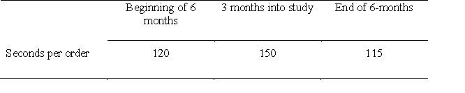 a. Create a line graph to represent the data presented in the table above.
b. Interpret this graph. What does it tell you?
c. Now that I have seen my results and they suggest that we got slower in the middle of the study, I want to know whether this slow-down was consistent across the different regions where we have restaurants. So suppose I divide the restaurants into those in the east coast of the United States and those on the west coast. I get the following results:
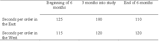 Create a line graph of these means.
d. What is the between-subjects variable in this mixed-model ANOVA?
e. Looking at the data presented in the table and figure above, do you think there is a time X region interaction on the dependent variable?
f. Suppose that the ANOVA results produced a value for the interaction between Time of Assessment and Seconds per order of F(2,98) = 4.36. Using an alpha level of .05, is this a statistically significant interaction?
a. Create a line graph to represent the data presented in the table above.b. Interpret this graph. What does it tell you?
c. Now that I have seen my results and they suggest that we got slower in the middle of the study, I want to know whether this slow-down was consistent across the different regions where we have restaurants. So suppose I divide the restaurants into those in the east coast of the United States and those on the west coast. I get the following results:
Create a line graph of these means.d. What is the between-subjects variable in this mixed-model ANOVA?
e. Looking at the data presented in the table and figure above, do you think there is a time X region interaction on the dependent variable?
f. Suppose that the ANOVA results produced a value for the interaction between Time of Assessment and Seconds per order of F(2,98) = 4.36. Using an alpha level of .05, is this a statistically significant interaction?

Unlock Deck
Sign up to unlock the cards in this deck!
Unlock Deck
Unlock Deck
1/3
Play
Full screen (f)
Deck 11: Repeated-Measures Analysis of Variance
What kind of question would be best examined with a repeated-measures ANOVA?
If I wanted to examine differences in the average scores of a sample over time or across trials. For example, if I wanted to determine whether a sample of high school students is more likely to use drugs before experiencing a drug-prevention course, right after finishing a drug-prevention course, or 6 months after finishing a drug prevention course, a repeated-measures ANOVA would be appropriate.
What kinds of variables are required to perform a mixed-model ANOVA that has both within-subject and between-subjects effects?
A dependent variable measured with an interval/ratio scale, at least one independent variable that is categorical/nominal (e.g., gender), and one variable that is measured at least twice for the within-subjects factor.
Suppose that I am the efficiency-control manager at a fast-food restaurant. Part of my job is to determine how long it takes to get orders to our customers. I want to know whether our efficiency changes across all 100 of our restaurants over a 6-month period. I collect data to figure out the average length of time it takes to get orders to customers at the beginning of the 6-month period, three months into the study period, and at the end of the 6-month period. I get the following data (in seconds per order):
a. Create a line graph to represent the data presented in the table above.
b. Interpret this graph. What does it tell you?
c. Now that I have seen my results and they suggest that we got slower in the middle of the study, I want to know whether this slow-down was consistent across the different regions where we have restaurants. So suppose I divide the restaurants into those in the east coast of the United States and those on the west coast. I get the following results:
Create a line graph of these means.
d. What is the between-subjects variable in this mixed-model ANOVA?
e. Looking at the data presented in the table and figure above, do you think there is a time X region interaction on the dependent variable?
f. Suppose that the ANOVA results produced a value for the interaction between Time of Assessment and Seconds per order of F(2,98) = 4.36. Using an alpha level of .05, is this a statistically significant interaction?
a. Create a line graph to represent the data presented in the table above.b. Interpret this graph. What does it tell you?
c. Now that I have seen my results and they suggest that we got slower in the middle of the study, I want to know whether this slow-down was consistent across the different regions where we have restaurants. So suppose I divide the restaurants into those in the east coast of the United States and those on the west coast. I get the following results:
Create a line graph of these means.d. What is the between-subjects variable in this mixed-model ANOVA?
e. Looking at the data presented in the table and figure above, do you think there is a time X region interaction on the dependent variable?
f. Suppose that the ANOVA results produced a value for the interaction between Time of Assessment and Seconds per order of F(2,98) = 4.36. Using an alpha level of .05, is this a statistically significant interaction?
a.
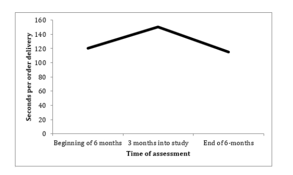 b. It appears that, on average across the 100 restaurants, it took longer to deliver orders to customers in the middle of the 6-month period of this study than it did at the beginning or the end. We would need to calulate the F value to determine whether this difference across the three time points is statistically significant.
c.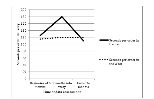 d. Region of the country that the restaurants were in.
e. The seconds-per-order in the West remained relatively flat across the three times of data collection, but in the East the seconds-per-order was higher in the second data-collection point than it was in the first or last data collection point.
f. Looking in Appendix C, with 2 and 100 degrees of freedom, the critical F value is 3.09. Because this critical F value is smaller than our observed F value of 4.36, we would conclude that this is a statistically significant interaction.
b. It appears that, on average across the 100 restaurants, it took longer to deliver orders to customers in the middle of the 6-month period of this study than it did at the beginning or the end. We would need to calulate the F value to determine whether this difference across the three time points is statistically significant.c.
d. Region of the country that the restaurants were in.e. The seconds-per-order in the West remained relatively flat across the three times of data collection, but in the East the seconds-per-order was higher in the second data-collection point than it was in the first or last data collection point.
f. Looking in Appendix C, with 2 and 100 degrees of freedom, the critical F value is 3.09. Because this critical F value is smaller than our observed F value of 4.36, we would conclude that this is a statistically significant interaction.
Unlock Deck
Unlock for access to all 3 flashcards in this deck.


