Deck 21: Inference for Regression
Full screen (f)
Question
A fisheries biologist has been studying horseshoe crabs using categorical variables, but she has decided that reporting the data as continuous variables would be more useful. She has sampled 100 horseshoe crabs and recorded their weight (in kilograms) and width (in centimeters). The proposed regression equation is
Weighti = α+β × widthi + Ɛi
Where the deviations Ɛi are assumed to be independent and Normally distributed with mean 0 and standard deviation σ. This model was fit to the data using the method of least squares. The following results were obtained from statistical software:
 r2 = 0.423, s = 2.2018.
What is the explanatory variable in this study?
A)Weight
B)Width
C)The slope, β
D)The intercept, α
Weighti = α+β × widthi + Ɛi
Where the deviations Ɛi are assumed to be independent and Normally distributed with mean 0 and standard deviation σ. This model was fit to the data using the method of least squares. The following results were obtained from statistical software:
r2 = 0.423, s = 2.2018.What is the explanatory variable in this study?
A)Weight
B)Width
C)The slope, β
D)The intercept, α
Question
A fisheries biologist has been studying horseshoe crabs using categorical variables, but she has decided that reporting the data as continuous variables would be more useful. She has sampled 100 horseshoe crabs and recorded their weight (in kilograms) and width (in centimeters). The proposed regression equation is
Weighti = α+β × widthi + Ɛi
Where the deviations Ɛi are assumed to be independent and Normally distributed with mean 0 and standard deviation σ. This model was fit to the data using the method of least squares. The following results were obtained from statistical software:
 r2 = 0.423, s = 2.2018.
The quantity s = 2.2018 is an estimate of the standard deviation, , of the deviations in the simple linear regression model. What is the degrees of freedom for s?
A)100
B)99
C)98
D)2
Weighti = α+β × widthi + Ɛi
Where the deviations Ɛi are assumed to be independent and Normally distributed with mean 0 and standard deviation σ. This model was fit to the data using the method of least squares. The following results were obtained from statistical software:
r2 = 0.423, s = 2.2018.The quantity s = 2.2018 is an estimate of the standard deviation, , of the deviations in the simple linear regression model. What is the degrees of freedom for s?
A)100
B)99
C)98
D)2
Question
A fisheries biologist has been studying horseshoe crabs using categorical variables, but she has decided that reporting the data as continuous variables would be more useful. She has sampled 100 horseshoe crabs and recorded their weight (in kilograms) and width (in centimeters). The proposed regression equation is
Weighti = α+β × widthi + Ɛi
Where the deviations Ɛi are assumed to be independent and Normally distributed with mean 0 and standard deviation σ. This model was fit to the data using the method of least squares. The following results were obtained from statistical software:
 r2 = 0.423, s = 2.2018.
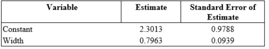
What is intercept of the least-squares regression line?
A)0.0939
B)0.7963
C)0.9788
D)2.3013
Weighti = α+β × widthi + Ɛi
Where the deviations Ɛi are assumed to be independent and Normally distributed with mean 0 and standard deviation σ. This model was fit to the data using the method of least squares. The following results were obtained from statistical software:
r2 = 0.423, s = 2.2018.What is intercept of the least-squares regression line?
A)0.0939
B)0.7963
C)0.9788
D)2.3013
Question
A fisheries biologist has been studying horseshoe crabs using categorical variables, but she has decided that reporting the data as continuous variables would be more useful. She has sampled 100 horseshoe crabs and recorded their weight (in kilograms) and width (in centimeters). The proposed regression equation is
Weighti = α+β × widthi + Ɛi
Where the deviations Ɛi are assumed to be independent and Normally distributed with mean 0 and standard deviation σ. This model was fit to the data using the method of least squares. The following results were obtained from statistical software:
 r2 = 0.423, s = 2.2018.
Suppose the researchers test the following hypotheses:
H0: = β=0, Hα: β> 0
What is the value of the t statistic for this test?
A)0.36
B)2.35
C)3.57
D)8.48
Weighti = α+β × widthi + Ɛi
Where the deviations Ɛi are assumed to be independent and Normally distributed with mean 0 and standard deviation σ. This model was fit to the data using the method of least squares. The following results were obtained from statistical software:
r2 = 0.423, s = 2.2018.Suppose the researchers test the following hypotheses:
H0: = β=0, Hα: β> 0
What is the value of the t statistic for this test?
A)0.36
B)2.35
C)3.57
D)8.48
Question
A fisheries biologist has been studying horseshoe crabs using categorical variables, but she has decided that reporting the data as continuous variables would be more useful. She has sampled 100 horseshoe crabs and recorded their weight (in kilograms) and width (in centimeters). The proposed regression equation is
Weighti = α+β × widthi + Ɛi
Where the deviations Ɛi are assumed to be independent and Normally distributed with mean 0 and standard deviation σ. This model was fit to the data using the method of least squares. The following results were obtained from statistical software:
 r2 = 0.423, s = 2.2018.
What is a 95% confidence interval for the slope in the simple linear regression model?
A)2.3013 ± 1.9419
B)2.3013 ± 0.1863
C)0.7963 ± 1.9419
D)0.7963 ± 0.1863
Weighti = α+β × widthi + Ɛi
Where the deviations Ɛi are assumed to be independent and Normally distributed with mean 0 and standard deviation σ. This model was fit to the data using the method of least squares. The following results were obtained from statistical software:
r2 = 0.423, s = 2.2018.What is a 95% confidence interval for the slope in the simple linear regression model?
A)2.3013 ± 1.9419
B)2.3013 ± 0.1863
C)0.7963 ± 1.9419
D)0.7963 ± 0.1863
Question
A fisheries biologist has been studying horseshoe crabs using categorical variables, but she has decided that reporting the data as continuous variables would be more useful. She has sampled 100 horseshoe crabs and recorded their weight (in kilograms) and width (in centimeters). The proposed regression equation is
Weighti = α+β × widthi + Ɛi
Where the deviations Ɛi are assumed to be independent and Normally distributed with mean 0 and standard deviation σ. This model was fit to the data using the method of least squares. The following results were obtained from statistical software:
 r2 = 0.423, s = 2.2018.
Based on the sample data, what is the correlation between the width and weight of horseshoe crabs?
A)-0.650
B)-0.423
C)0.423
D)0.650
Weighti = α+β × widthi + Ɛi
Where the deviations Ɛi are assumed to be independent and Normally distributed with mean 0 and standard deviation σ. This model was fit to the data using the method of least squares. The following results were obtained from statistical software:
r2 = 0.423, s = 2.2018.Based on the sample data, what is the correlation between the width and weight of horseshoe crabs?
A)-0.650
B)-0.423
C)0.423
D)0.650
Question
Question
Question
Question
Question
Question
Question
Question
Data on the water quality in the eastern United States were obtained by a researcher who wanted to ascertain whether the amount of particulates in water (ppm) could be used to accurately predict the water quality score. Suppose we use the following simple linear regression model:
Qualityi = α+ β× particulatesi + Ɛi
Where the deviations Ɛi are assumed to be independent and Normally distributed with mean 0 and standard deviation σ. This model was fit to the data using the method of least squares. The following results were obtained from statistical software based on a sample of size 61:
r2 = 0.005, s = 0.7896.
Here is a scatterplot of the amount of particulates versus water quality:
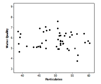 Which of the following statements is supported by the plot?
A)There is no striking evidence in the plot suggesting that the assumptions for regression are violated.
B)There appears to be a serious outlier in the plot, suggesting that our results must be interpreted with caution.
C)The plot contains dramatic evidence that the standard deviation of the response about the true regression line is not approximately the same everywhere.
D)The plot contains many fewer points than were used to fit the least-squares regression line in the previous problems.Obviously, there is a major error present.
Qualityi = α+ β× particulatesi + Ɛi
Where the deviations Ɛi are assumed to be independent and Normally distributed with mean 0 and standard deviation σ. This model was fit to the data using the method of least squares. The following results were obtained from statistical software based on a sample of size 61:
r2 = 0.005, s = 0.7896.
Here is a scatterplot of the amount of particulates versus water quality:
Which of the following statements is supported by the plot?A)There is no striking evidence in the plot suggesting that the assumptions for regression are violated.
B)There appears to be a serious outlier in the plot, suggesting that our results must be interpreted with caution.
C)The plot contains dramatic evidence that the standard deviation of the response about the true regression line is not approximately the same everywhere.
D)The plot contains many fewer points than were used to fit the least-squares regression line in the previous problems.Obviously, there is a major error present.
Question
Question
Question
Question
Question
Question
Question
Question
Question
Question
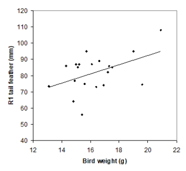
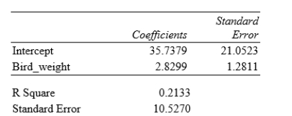
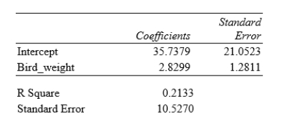
Tail-feather length in birds is sometimes a sexually dimorphic trait; that is, the trait differs substantially for males and for females of the same species. Researchers studied the relationship between tail-feather length (measuring the R1 central tail feather) and weight in a sample of 20 male long-tailed finches raised in an aviary. The data are displayed in the scatterplot below, followed with software output about the least-squares regression model of feather length as a function of weight.

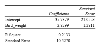 What is the value of the slope for the least-squares regression line?
A)21.0523
B)2.8299
C)35.7379
D)1.2811
What is the value of the slope for the least-squares regression line?A)21.0523
B)2.8299
C)35.7379
D)1.2811
Question
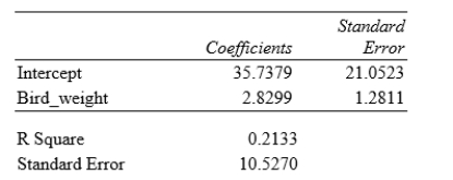
Tail-feather length in birds is sometimes a sexually dimorphic trait; that is, the trait differs substantially for males and for females of the same species. Researchers studied the relationship between tail-feather length (measuring the R1 central tail feather) and weight in a sample of 20 male long-tailed finches raised in an aviary. The data are displayed in the scatterplot below, followed with software output about the least-squares regression model of feather length as a function of weight.

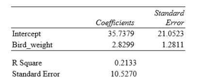 What does the standard error value of 10.5270 represent?
A)An estimate of the standard deviation σof the deviations about the mean in the linear regression model
B)The population standard deviationσ of the deviations about the mean in the linear regression model
C)The sample standard deviation of the feather lengths
D)The sample standard deviation of the feather lengths divided by √n
What does the standard error value of 10.5270 represent?A)An estimate of the standard deviation σof the deviations about the mean in the linear regression model
B)The population standard deviationσ of the deviations about the mean in the linear regression model
C)The sample standard deviation of the feather lengths
D)The sample standard deviation of the feather lengths divided by √n
Question
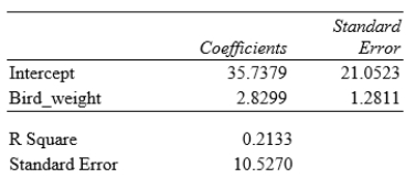
Tail-feather length in birds is sometimes a sexually dimorphic trait; that is, the trait differs substantially for males and for females of the same species. Researchers studied the relationship between tail-feather length (measuring the R1 central tail feather) and weight in a sample of 20 male long-tailed finches raised in an aviary. The data are displayed in the scatterplot below, followed with software output about the least-squares regression model of feather length as a function of weight.
 What percentage of variation in tail-feather length that can be explained by this linear model?
A)5%
B)21%
C)46%
D)79%
What percentage of variation in tail-feather length that can be explained by this linear model?A)5%
B)21%
C)46%
D)79%
Question
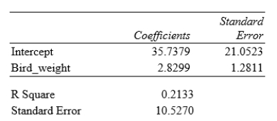
Tail-feather length in birds is sometimes a sexually dimorphic trait; that is, the trait differs substantially for males and for females of the same species. Researchers studied the relationship between tail-feather length (measuring the R1 central tail feather) and weight in a sample of 20 male long-tailed finches raised in an aviary. The data are displayed in the scatterplot below, followed with software output about the least-squares regression model of feather length as a function of weight.

 We want to test the hypotheses H0: β = 0 versus Ha: β > 0, where β is the true value of the population slope. What is the value of the t statistic for this test?
A)1.28
B)1.70
C)2.21
D)2.83
We want to test the hypotheses H0: β = 0 versus Ha: β > 0, where β is the true value of the population slope. What is the value of the t statistic for this test?A)1.28
B)1.70
C)2.21
D)2.83
Question
Tail-feather length in birds is sometimes a sexually dimorphic trait; that is, the trait differs substantially for males and for females of the same species. Researchers studied the relationship between tail-feather length (measuring the R1 central tail feather) and weight in a sample of 20 male long-tailed finches raised in an aviary. The data are displayed in the scatterplot below, followed with software output about the least-squares regression model of feather length as a function of weight.

 We want to test the hypotheses H0: β = 0 versus Ha: β > 0, where β is the true value of the population slope. What is the P-value for this test?
A)Less than 0.01
B)Between 0.01 and 0.05
C)Between 0.05 and 0.10
D)Greater than 0.10
We want to test the hypotheses H0: β = 0 versus Ha: β > 0, where β is the true value of the population slope. What is the P-value for this test?A)Less than 0.01
B)Between 0.01 and 0.05
C)Between 0.05 and 0.10
D)Greater than 0.10
Question
Tail-feather length in birds is sometimes a sexually dimorphic trait; that is, the trait differs substantially for males and for females of the same species. Researchers studied the relationship between tail-feather length (measuring the R1 central tail feather) and weight in a sample of 20 male long-tailed finches raised in an aviary. The data are displayed in the scatterplot below, followed with software output about the least-squares regression model of feather length as a function of weight.

 What is the margin of error for a 95% confidence interval for the true population slope β in this linear regression model?
A)1.28
B)2.10
C)2.51
D)2.69
What is the margin of error for a 95% confidence interval for the true population slope β in this linear regression model?A)1.28
B)2.10
C)2.51
D)2.69
Question
Tail-feather length in birds is sometimes a sexually dimorphic trait; that is, the trait differs substantially for males and for females of the same species. Researchers studied the relationship between tail-feather length (measuring the R1 central tail feather) and weight in a sample of 20 male long-tailed finches raised in an aviary. The data are displayed in the scatterplot below, followed with software output about the least-squares regression model of feather length as a function of weight.

 Which of the following conclusions best describes the findings?
A)There is no evidence (P > 0.10) of a linear relationship between tail-feather length and weight in male long-tailed finches.
B)There is weak evidence (0.05 < P < 0.10) of a linear relationship between tail-feather length and weight in male long-tailed finches.
C)There is significant evidence (P < 0.05) of a positive linear relationship between tail-feather length and weight in male long-tailed finches.
D)There is significant evidence (P < 0.05) that there is no linear relationship between tail-feather length and weight in male long-tailed finches.
Which of the following conclusions best describes the findings?A)There is no evidence (P > 0.10) of a linear relationship between tail-feather length and weight in male long-tailed finches.
B)There is weak evidence (0.05 < P < 0.10) of a linear relationship between tail-feather length and weight in male long-tailed finches.
C)There is significant evidence (P < 0.05) of a positive linear relationship between tail-feather length and weight in male long-tailed finches.
D)There is significant evidence (P < 0.05) that there is no linear relationship between tail-feather length and weight in male long-tailed finches.
Question
Question
Question
Question
Question
Question
Question
Question
Question
Question
Question
Researchers want to know if reading skills can explain IQ test scores in children with dyslexia. The following scatterplot examines the relationship between reading skill score and IQ test score for 22 dyslexic children. The least-squares regression line is displayed on the plot, along with the value of r2.
 We want to test a hypothesis of no relationship between the two scores, H0: p= 0 versus Ha: p≠0.
What is the P-value for this test?
A)Less than 0.01
B)Between 0.01 and 0.05
C)Between 0.05 and 0.10
D)Greater than 0.10
We want to test a hypothesis of no relationship between the two scores, H0: p= 0 versus Ha: p≠0.What is the P-value for this test?
A)Less than 0.01
B)Between 0.01 and 0.05
C)Between 0.05 and 0.10
D)Greater than 0.10
Question
Researchers want to know if reading skills can explain IQ test scores in children with dyslexia. The following scatterplot examines the relationship between reading skill score and IQ test score for 22 dyslexic children. The least-squares regression line is displayed on the plot, along with the value of r2.
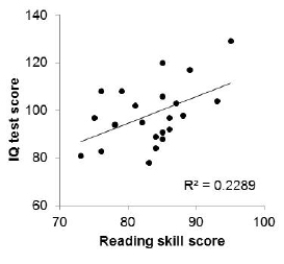 Here is software output for predicting IQ test score when reading skill score = 80:
What is the best description of the interval (69.44, 119.74)?
A)95% confidence interval for the IQ test score of a dyslexic child with a reading skill score of 80
B)95% prediction interval for the IQ test score of a dyslexic child with a reading skill score of 80
C)95% confidence interval for the mean IQ test score of all dyslexic children with a reading skill score of 80
D)95% prediction interval for the mean IQ test score of all dyslexic children with a reading skill score of 80
Here is software output for predicting IQ test score when reading skill score = 80:What is the best description of the interval (69.44, 119.74)?
A)95% confidence interval for the IQ test score of a dyslexic child with a reading skill score of 80
B)95% prediction interval for the IQ test score of a dyslexic child with a reading skill score of 80
C)95% confidence interval for the mean IQ test score of all dyslexic children with a reading skill score of 80
D)95% prediction interval for the mean IQ test score of all dyslexic children with a reading skill score of 80
Question
Question
Question

Unlock Deck
Sign up to unlock the cards in this deck!
Unlock Deck
Unlock Deck
1/45
Play
Full screen (f)
Deck 21: Inference for Regression
1
A fisheries biologist has been studying horseshoe crabs using categorical variables, but she has decided that reporting the data as continuous variables would be more useful. She has sampled 100 horseshoe crabs and recorded their weight (in kilograms) and width (in centimeters). The proposed regression equation is
Weighti = α+β × widthi + Ɛi
Where the deviations Ɛi are assumed to be independent and Normally distributed with mean 0 and standard deviation σ. This model was fit to the data using the method of least squares. The following results were obtained from statistical software:
r2 = 0.423, s = 2.2018.
What is the explanatory variable in this study?
A)Weight
B)Width
C)The slope, β
D)The intercept, α
Weighti = α+β × widthi + Ɛi
Where the deviations Ɛi are assumed to be independent and Normally distributed with mean 0 and standard deviation σ. This model was fit to the data using the method of least squares. The following results were obtained from statistical software:
r2 = 0.423, s = 2.2018.What is the explanatory variable in this study?
A)Weight
B)Width
C)The slope, β
D)The intercept, α
B
2
A fisheries biologist has been studying horseshoe crabs using categorical variables, but she has decided that reporting the data as continuous variables would be more useful. She has sampled 100 horseshoe crabs and recorded their weight (in kilograms) and width (in centimeters). The proposed regression equation is
Weighti = α+β × widthi + Ɛi
Where the deviations Ɛi are assumed to be independent and Normally distributed with mean 0 and standard deviation σ. This model was fit to the data using the method of least squares. The following results were obtained from statistical software:
r2 = 0.423, s = 2.2018.
The quantity s = 2.2018 is an estimate of the standard deviation, , of the deviations in the simple linear regression model. What is the degrees of freedom for s?
A)100
B)99
C)98
D)2
Weighti = α+β × widthi + Ɛi
Where the deviations Ɛi are assumed to be independent and Normally distributed with mean 0 and standard deviation σ. This model was fit to the data using the method of least squares. The following results were obtained from statistical software:
r2 = 0.423, s = 2.2018.The quantity s = 2.2018 is an estimate of the standard deviation, , of the deviations in the simple linear regression model. What is the degrees of freedom for s?
A)100
B)99
C)98
D)2
C
3
A fisheries biologist has been studying horseshoe crabs using categorical variables, but she has decided that reporting the data as continuous variables would be more useful. She has sampled 100 horseshoe crabs and recorded their weight (in kilograms) and width (in centimeters). The proposed regression equation is
Weighti = α+β × widthi + Ɛi
Where the deviations Ɛi are assumed to be independent and Normally distributed with mean 0 and standard deviation σ. This model was fit to the data using the method of least squares. The following results were obtained from statistical software:
r2 = 0.423, s = 2.2018.
What is intercept of the least-squares regression line?
A)0.0939
B)0.7963
C)0.9788
D)2.3013
Weighti = α+β × widthi + Ɛi
Where the deviations Ɛi are assumed to be independent and Normally distributed with mean 0 and standard deviation σ. This model was fit to the data using the method of least squares. The following results were obtained from statistical software:
r2 = 0.423, s = 2.2018.What is intercept of the least-squares regression line?
A)0.0939
B)0.7963
C)0.9788
D)2.3013
D
4
A fisheries biologist has been studying horseshoe crabs using categorical variables, but she has decided that reporting the data as continuous variables would be more useful. She has sampled 100 horseshoe crabs and recorded their weight (in kilograms) and width (in centimeters). The proposed regression equation is
Weighti = α+β × widthi + Ɛi
Where the deviations Ɛi are assumed to be independent and Normally distributed with mean 0 and standard deviation σ. This model was fit to the data using the method of least squares. The following results were obtained from statistical software:
r2 = 0.423, s = 2.2018.
Suppose the researchers test the following hypotheses:
H0: = β=0, Hα: β> 0
What is the value of the t statistic for this test?
A)0.36
B)2.35
C)3.57
D)8.48
Weighti = α+β × widthi + Ɛi
Where the deviations Ɛi are assumed to be independent and Normally distributed with mean 0 and standard deviation σ. This model was fit to the data using the method of least squares. The following results were obtained from statistical software:
r2 = 0.423, s = 2.2018.Suppose the researchers test the following hypotheses:
H0: = β=0, Hα: β> 0
What is the value of the t statistic for this test?
A)0.36
B)2.35
C)3.57
D)8.48
Unlock Deck
Unlock for access to all 45 flashcards in this deck.
Unlock Deck
k this deck
5
A fisheries biologist has been studying horseshoe crabs using categorical variables, but she has decided that reporting the data as continuous variables would be more useful. She has sampled 100 horseshoe crabs and recorded their weight (in kilograms) and width (in centimeters). The proposed regression equation is
Weighti = α+β × widthi + Ɛi
Where the deviations Ɛi are assumed to be independent and Normally distributed with mean 0 and standard deviation σ. This model was fit to the data using the method of least squares. The following results were obtained from statistical software:
r2 = 0.423, s = 2.2018.
What is a 95% confidence interval for the slope in the simple linear regression model?
A)2.3013 ± 1.9419
B)2.3013 ± 0.1863
C)0.7963 ± 1.9419
D)0.7963 ± 0.1863
Weighti = α+β × widthi + Ɛi
Where the deviations Ɛi are assumed to be independent and Normally distributed with mean 0 and standard deviation σ. This model was fit to the data using the method of least squares. The following results were obtained from statistical software:
r2 = 0.423, s = 2.2018.What is a 95% confidence interval for the slope in the simple linear regression model?
A)2.3013 ± 1.9419
B)2.3013 ± 0.1863
C)0.7963 ± 1.9419
D)0.7963 ± 0.1863
Unlock Deck
Unlock for access to all 45 flashcards in this deck.
Unlock Deck
k this deck
6
A fisheries biologist has been studying horseshoe crabs using categorical variables, but she has decided that reporting the data as continuous variables would be more useful. She has sampled 100 horseshoe crabs and recorded their weight (in kilograms) and width (in centimeters). The proposed regression equation is
Weighti = α+β × widthi + Ɛi
Where the deviations Ɛi are assumed to be independent and Normally distributed with mean 0 and standard deviation σ. This model was fit to the data using the method of least squares. The following results were obtained from statistical software:
r2 = 0.423, s = 2.2018.
Based on the sample data, what is the correlation between the width and weight of horseshoe crabs?
A)-0.650
B)-0.423
C)0.423
D)0.650
Weighti = α+β × widthi + Ɛi
Where the deviations Ɛi are assumed to be independent and Normally distributed with mean 0 and standard deviation σ. This model was fit to the data using the method of least squares. The following results were obtained from statistical software:
r2 = 0.423, s = 2.2018.Based on the sample data, what is the correlation between the width and weight of horseshoe crabs?
A)-0.650
B)-0.423
C)0.423
D)0.650
Unlock Deck
Unlock for access to all 45 flashcards in this deck.
Unlock Deck
k this deck
7
A fisheries biologist has been studying horseshoe crabs using categorical variables, but she has decided that reporting the data as continuous variables would be more useful. She has sampled 100 horseshoe crabs and recorded their weight (in kilograms) and width (in centimeters). The proposed regression equation is weighti = α+β × widthi + Ɛi
Where the deviations Ɛi are assumed to be independent and Normally distributed with mean 0 and standard deviation σ . This model was fit to the data using the method of least squares. The following results were obtained from statistical software:
r2 = 0.423, s = 2.2018.
Suppose we use statistical software to predict the weight for a horseshoe crab with width 2.25 centimeters, which yields the following:
What is a 95% confidence interval for this prediction according to this output?
A)(2.556, 5.630)
B)(-0.539, 8.725)
C)4.093 ± 1.9419
D)4.093 ± 0.1863
Unlock Deck
Unlock for access to all 45 flashcards in this deck.
Unlock Deck
k this deck
8
A fisheries biologist has been studying horseshoe crabs using categorical variables, but she has decided that reporting the data as continuous variables would be more useful. She has sampled 100 horseshoe crabs and recorded their weight (in kilograms) and width (in centimeters). The proposed regression equation is weighti = α+β × widthi + Ɛi
Where the deviations Ɛi are assumed to be independent and Normally distributed with mean 0 and standard deviation σ . This model was fit to the data using the method of least squares. The following results were obtained from statistical software:
r2 = 0.423, s = 2.2018.
Suppose we use statistical software to predict the weight for a horseshoe crab with width 2.25 centimeters, which yields the following:
What is a 95% interval for this prediction according to this output?
A)(2.556, 5.630)
B)(-0.539, 8.725)
C)4.093 ± 1.9419
D)4.093 ± 0.1863
Unlock Deck
Unlock for access to all 45 flashcards in this deck.
Unlock Deck
k this deck
9
Data on the water quality in the eastern United States were obtained by a researcher who wanted to ascertain whether the amount of particulates in water (ppm) could be used to accurately predict the water quality score. Suppose we use the following simple linear regression model:
Qualityi = α+ β× particulatesi + Ɛi
Where the deviations Ɛi are assumed to be independent and Normally distributed with mean 0 and standard deviation σ. This model was fit to the data using the method of least squares. The following results were obtained from statistical software based on a sample of size 61:
r2 = 0.005, s = 0.7896.
What is the intercept of the least-squares regression line?
A)-0.009
B)0.020
C)1.003
D)6.214
Unlock Deck
Unlock for access to all 45 flashcards in this deck.
Unlock Deck
k this deck
10
Data on the water quality in the eastern United States were obtained by a researcher who wanted to ascertain whether the amount of particulates in water (ppm) could be used to accurately predict the water quality score. Suppose we use the following simple linear regression model:
Qualityi = α+ β× particulatesi + Ɛi
Where the deviations Ɛi are assumed to be independent and Normally distributed with mean 0 and standard deviation σ. This model was fit to the data using the method of least squares. The following results were obtained from statistical software based on a sample of size 61:
r2 = 0.005, s = 0.7896.
What is a 90% confidence interval for the slope in the simple linear regression model?
A)-0.009 ± 0.0334
B)-0.009 ± 1.6820
C)6.214 ± 0.0334
D)6.214 ± 1.6820
Unlock Deck
Unlock for access to all 45 flashcards in this deck.
Unlock Deck
k this deck
11
Data on the water quality in the eastern United States were obtained by a researcher who wanted to ascertain whether the amount of particulates in water (ppm) could be used to accurately predict the water quality score. Suppose we use the following simple linear regression model:
Qualityi = α+ β× particulatesi + Ɛi
Where the deviations Ɛi are assumed to be independent and Normally distributed with mean 0 and standard deviation σ. This model was fit to the data using the method of least squares. The following results were obtained from statistical software based on a sample of size 61:
r2 = 0.005, s = 0.7896.
Suppose the researcher tests the following hypotheses:
H0: β1 = 0, Ha: β1 0
What is the value of the t statistic for this test?
A)-6.20
B)-0.45
C)0.45
D)6.20
Unlock Deck
Unlock for access to all 45 flashcards in this deck.
Unlock Deck
k this deck
12
Data on the water quality in the eastern United States were obtained by a researcher who wanted to ascertain whether the amount of particulates in water (ppm) could be used to accurately predict the water quality score. Suppose we use the following simple linear regression model:
Qualityi = α+ β× particulatesi + Ɛi
Where the deviations Ɛi are assumed to be independent and Normally distributed with mean 0 and standard deviation σ. This model was fit to the data using the method of least squares. The following results were obtained from statistical software based on a sample of size 61:
r2 = 0.005, s = 0.7896.
What is the correlation between the amount of particulates and water quality?
A)-0.005
B)-0.071
C)0.071
D)0.005
Unlock Deck
Unlock for access to all 45 flashcards in this deck.
Unlock Deck
k this deck
13
Data on the water quality in the eastern United States were obtained by a researcher who wanted to ascertain whether the amount of particulates in water (ppm) could be used to accurately predict the water quality score. Suppose we use the following simple linear regression model:
Qualityi = α+ β× particulatesi + Ɛi
Where the deviations Ɛi are assumed to be independent and Normally distributed with mean 0 and standard deviation σ. This model was fit to the data using the method of least squares. The following results were obtained from statistical software based on a sample of size 61:
r2 = 0.005, s = 0.7896.
Is there strong evidence (and if so, why?) that there is a straight-line dependence between the amount of particulates and water quality?
A)Yes, because the slope of the least-squares line is not zero.
B)Yes, because the confidence interval for the slope includes zero.
C)No, because the confidence interval for the slope includes zero.
D)It is impossible to say because we are not given the actual value of the correlation.
Unlock Deck
Unlock for access to all 45 flashcards in this deck.
Unlock Deck
k this deck
14
Data on the water quality in the eastern United States were obtained by a researcher who wanted to ascertain whether the amount of particulates in water (ppm) could be used to accurately predict the water quality score. Suppose we use the following simple linear regression model:
Qualityi = α+ β× particulatesi + Ɛi
Where the deviations Ɛi are assumed to be independent and Normally distributed with mean 0 and standard deviation σ. This model was fit to the data using the method of least squares. The following results were obtained from statistical software based on a sample of size 61:
r2 = 0.005, s = 0.7896.
Here is a scatterplot of the amount of particulates versus water quality:
Which of the following statements is supported by the plot?
A)There is no striking evidence in the plot suggesting that the assumptions for regression are violated.
B)There appears to be a serious outlier in the plot, suggesting that our results must be interpreted with caution.
C)The plot contains dramatic evidence that the standard deviation of the response about the true regression line is not approximately the same everywhere.
D)The plot contains many fewer points than were used to fit the least-squares regression line in the previous problems.Obviously, there is a major error present.
Qualityi = α+ β× particulatesi + Ɛi
Where the deviations Ɛi are assumed to be independent and Normally distributed with mean 0 and standard deviation σ. This model was fit to the data using the method of least squares. The following results were obtained from statistical software based on a sample of size 61:
r2 = 0.005, s = 0.7896.
Here is a scatterplot of the amount of particulates versus water quality:
Which of the following statements is supported by the plot?A)There is no striking evidence in the plot suggesting that the assumptions for regression are violated.
B)There appears to be a serious outlier in the plot, suggesting that our results must be interpreted with caution.
C)The plot contains dramatic evidence that the standard deviation of the response about the true regression line is not approximately the same everywhere.
D)The plot contains many fewer points than were used to fit the least-squares regression line in the previous problems.Obviously, there is a major error present.
Unlock Deck
Unlock for access to all 45 flashcards in this deck.
Unlock Deck
k this deck
15
A random sample of 79 patients from a walk-in clinic records the low- and high-density cholesterol levels of the patients, labeled LDL and HDL, respectively. LDL is often referred to as "bad" cholesterol, while HDL is often referred to as "good" cholesterol. A researcher is interested in fitting the following linear regression curve to LDL and HDL levels:
LDLi = α+ β× HDLi + Ɛi
Where the deviations i are assumed to be independent and Normally distributed with mean 0 and standard deviation . This model was fit to the data using the method of least squares. The following results were obtained from statistical software:
r2 = 0.810, s = 50.
What is the intercept of the least-squares regression line?
A)0.025
B)0.75
C)3
D)-25
Unlock Deck
Unlock for access to all 45 flashcards in this deck.
Unlock Deck
k this deck
16
A random sample of 79 patients from a walk-in clinic records the low- and high-density cholesterol levels of the patients, labeled LDL and HDL, respectively. LDL is often referred to as "bad" cholesterol, while HDL is often referred to as "good" cholesterol. A researcher is interested in fitting the following linear regression curve to LDL and HDL levels:
LDLi = α+ β× HDLi + Ɛi
Where the deviations Ɛi are assumed to be independent and Normally distributed with mean 0 and standard deviation σ. This model was fit to the data using the method of least squares. The following results were obtained from statistical software:
r2 = 0.810, s = 50.
What is a 90% confidence interval for the slope β1 in the simple linear regression model?
A)0.75 ± 4.995
B)0.75 ± 0.042
C)-25 ± 4.995
D)-25 ± 0.042
Unlock Deck
Unlock for access to all 45 flashcards in this deck.
Unlock Deck
k this deck
17
A random sample of 79 patients from a walk-in clinic records the low- and high-density cholesterol levels of the patients, labeled LDL and HDL, respectively. LDL is often referred to as "bad" cholesterol, while HDL is often referred to as "good" cholesterol. A researcher is interested in fitting the following linear regression curve to LDL and HDL levels:
LDLi = α+ β× HDLi + Ɛi
Where the deviations Ɛi are assumed to be independent and Normally distributed with mean 0 and standard deviation σ. This model was fit to the data using the method of least squares. The following results were obtained from statistical software:
r2 = 0.810, s = 50.
Suppose the researchers test the following hypotheses:
H0: β1 = 0, Ha: β1 > 0
What is the P-value of the test?
A)Greater than 0.10
B)Between 0.10 and 0.05
C)Between 0.05 and 0.01
D)Less than 0.01
Unlock Deck
Unlock for access to all 45 flashcards in this deck.
Unlock Deck
k this deck
18
A random sample of 79 patients from a walk-in clinic records the low- and high-density cholesterol levels of the patients, labeled LDL and HDL, respectively. LDL is often referred to as "bad" cholesterol, while HDL is often referred to as "good" cholesterol. A researcher is interested in fitting the following linear regression curve to LDL and HDL levels:
LDLi = α+ β× HDLi + Ɛi
Where the deviations Ɛi are assumed to be independent and Normally distributed with mean 0 and standard deviation σ. This model was fit to the data using the method of least squares. The following results were obtained from statistical software:
r2 = 0.810, s = 50.
Is there strong evidence (and if so, why?) of a straight-line relationship between LDL and HDL?
A)Yes, because the slope of the least-squares line is positive.
B)Yes, because the P-value for testing whether the slope is 0 is quite small.
C)No, because the value of the square of the correlation is relatively small.
D)It is impossible to say because we are not given the actual value of the correlation.
Unlock Deck
Unlock for access to all 45 flashcards in this deck.
Unlock Deck
k this deck
19
Tail-feather length in birds is sometimes a sexually dimorphic trait; that is, the trait differs substantially for males and for females. Researchers studied the relationship between weight (x) and tail-feather length (y) in a sample of 5 wild male long-tailed finches. Here are the data:
Using appropriate software to perform the necessary calculations, what does the value of the slope for the least-squares regression line tells us?
A)For every 1 g change in weight, tail length increases by 0.280 mm, on average.
B)For every 1 g change in weight, tail length increases by 2.81 mm, on average.
C)For every 1g change in weight, tail length increases by 0.789 mm, on average.
D)For every 1 g change in weight, tail length increases by 25.547 mm, on average.
Unlock Deck
Unlock for access to all 45 flashcards in this deck.
Unlock Deck
k this deck
20
Tail-feather length in birds is sometimes a sexually dimorphic trait; that is, the trait differs substantially for males and for females. Researchers studied the relationship between weight (x) and tail-feather length (y) in a sample of 5 wild male long-tailed finches. Here are the data:
Using appropriate software, what is the numerical value of the y intercept for the least-squares regression line?
A)0.280
B)2.815
C)3.741
D)25.547
Using appropriate software, what is the numerical value of the y intercept for the least-squares regression line?
A)0.280
B)2.815
C)3.741
D)25.547
Unlock Deck
Unlock for access to all 45 flashcards in this deck.
Unlock Deck
k this deck
21
Tail-feather length in birds is sometimes a sexually dimorphic trait; that is, the trait differs substantially for males and for females. Researchers studied the relationship between weight (x) and tail-feather length (y) in a sample of 5 wild male long-tailed finches. Here are the data:
Using appropriate software, what percentage of variation in tail-feather length can be explained by weight among male long-tailed finches in the wild?
A)62%
B)79%
C)89%
D)94%
Using appropriate software, what percentage of variation in tail-feather length can be explained by weight among male long-tailed finches in the wild?
A)62%
B)79%
C)89%
D)94%
Unlock Deck
Unlock for access to all 45 flashcards in this deck.
Unlock Deck
k this deck
22
Tail-feather length in birds is sometimes a sexually dimorphic trait; that is, the trait differs substantially for males and for females. Researchers studied the relationship between weight (x) and tail-feather length (y) in a sample of 5 wild male long-tailed finches. Here are the data:
We want to test the hypotheses H0: β= 0, versus Ha: β> 0, where βis the true value of the population slope. Using appropriate software, what is the value of the t statistic for this test?
A)0.89
B)2.81
C)3.34
D)3.74
We want to test the hypotheses H0: β= 0, versus Ha: β> 0, where βis the true value of the population slope. Using appropriate software, what is the value of the t statistic for this test?
A)0.89
B)2.81
C)3.34
D)3.74
Unlock Deck
Unlock for access to all 45 flashcards in this deck.
Unlock Deck
k this deck
23
Tail-feather length in birds is sometimes a sexually dimorphic trait; that is, the trait differs substantially for males and for females. Researchers studied the relationship between weight (x) and tail-feather length (y) in a sample of 5 wild male long-tailed finches. Here are the data:
We want to test the hypotheses H0: β= 0, versus Ha: β> 0, where βis the true value of the population slope. Using appropriate software, what is the P-value for this test?
A)Less than 0.01
B)Between 0.01 and 0.05
C)Between 0.05 and 0.10
D)Greater than 0.10
We want to test the hypotheses H0: β= 0, versus Ha: β> 0, where βis the true value of the population slope. Using appropriate software, what is the P-value for this test?
A)Less than 0.01
B)Between 0.01 and 0.05
C)Between 0.05 and 0.10
D)Greater than 0.10
Unlock Deck
Unlock for access to all 45 flashcards in this deck.
Unlock Deck
k this deck
24
Tail-feather length in birds is sometimes a sexually dimorphic trait; that is, the trait differs substantially for males and for females of the same species. Researchers studied the relationship between tail-feather length (measuring the R1 central tail feather) and weight in a sample of 20 male long-tailed finches raised in an aviary. The data are displayed in the scatterplot below, followed with software output about the least-squares regression model of feather length as a function of weight.
What is the value of the slope for the least-squares regression line?
A)21.0523
B)2.8299
C)35.7379
D)1.2811
What is the value of the slope for the least-squares regression line?A)21.0523
B)2.8299
C)35.7379
D)1.2811
Unlock Deck
Unlock for access to all 45 flashcards in this deck.
Unlock Deck
k this deck
25
Tail-feather length in birds is sometimes a sexually dimorphic trait; that is, the trait differs substantially for males and for females of the same species. Researchers studied the relationship between tail-feather length (measuring the R1 central tail feather) and weight in a sample of 20 male long-tailed finches raised in an aviary. The data are displayed in the scatterplot below, followed with software output about the least-squares regression model of feather length as a function of weight.
What does the standard error value of 10.5270 represent?
A)An estimate of the standard deviation σof the deviations about the mean in the linear regression model
B)The population standard deviationσ of the deviations about the mean in the linear regression model
C)The sample standard deviation of the feather lengths
D)The sample standard deviation of the feather lengths divided by √n
What does the standard error value of 10.5270 represent?A)An estimate of the standard deviation σof the deviations about the mean in the linear regression model
B)The population standard deviationσ of the deviations about the mean in the linear regression model
C)The sample standard deviation of the feather lengths
D)The sample standard deviation of the feather lengths divided by √n
Unlock Deck
Unlock for access to all 45 flashcards in this deck.
Unlock Deck
k this deck
26
Tail-feather length in birds is sometimes a sexually dimorphic trait; that is, the trait differs substantially for males and for females of the same species. Researchers studied the relationship between tail-feather length (measuring the R1 central tail feather) and weight in a sample of 20 male long-tailed finches raised in an aviary. The data are displayed in the scatterplot below, followed with software output about the least-squares regression model of feather length as a function of weight.
What percentage of variation in tail-feather length that can be explained by this linear model?
A)5%
B)21%
C)46%
D)79%
What percentage of variation in tail-feather length that can be explained by this linear model?A)5%
B)21%
C)46%
D)79%
Unlock Deck
Unlock for access to all 45 flashcards in this deck.
Unlock Deck
k this deck
27
Tail-feather length in birds is sometimes a sexually dimorphic trait; that is, the trait differs substantially for males and for females of the same species. Researchers studied the relationship between tail-feather length (measuring the R1 central tail feather) and weight in a sample of 20 male long-tailed finches raised in an aviary. The data are displayed in the scatterplot below, followed with software output about the least-squares regression model of feather length as a function of weight.
We want to test the hypotheses H0: β = 0 versus Ha: β > 0, where β is the true value of the population slope. What is the value of the t statistic for this test?
A)1.28
B)1.70
C)2.21
D)2.83
We want to test the hypotheses H0: β = 0 versus Ha: β > 0, where β is the true value of the population slope. What is the value of the t statistic for this test?A)1.28
B)1.70
C)2.21
D)2.83
Unlock Deck
Unlock for access to all 45 flashcards in this deck.
Unlock Deck
k this deck
28
Tail-feather length in birds is sometimes a sexually dimorphic trait; that is, the trait differs substantially for males and for females of the same species. Researchers studied the relationship between tail-feather length (measuring the R1 central tail feather) and weight in a sample of 20 male long-tailed finches raised in an aviary. The data are displayed in the scatterplot below, followed with software output about the least-squares regression model of feather length as a function of weight.
We want to test the hypotheses H0: β = 0 versus Ha: β > 0, where β is the true value of the population slope. What is the P-value for this test?
A)Less than 0.01
B)Between 0.01 and 0.05
C)Between 0.05 and 0.10
D)Greater than 0.10
We want to test the hypotheses H0: β = 0 versus Ha: β > 0, where β is the true value of the population slope. What is the P-value for this test?A)Less than 0.01
B)Between 0.01 and 0.05
C)Between 0.05 and 0.10
D)Greater than 0.10
Unlock Deck
Unlock for access to all 45 flashcards in this deck.
Unlock Deck
k this deck
29
Tail-feather length in birds is sometimes a sexually dimorphic trait; that is, the trait differs substantially for males and for females of the same species. Researchers studied the relationship between tail-feather length (measuring the R1 central tail feather) and weight in a sample of 20 male long-tailed finches raised in an aviary. The data are displayed in the scatterplot below, followed with software output about the least-squares regression model of feather length as a function of weight.
What is the margin of error for a 95% confidence interval for the true population slope β in this linear regression model?
A)1.28
B)2.10
C)2.51
D)2.69
What is the margin of error for a 95% confidence interval for the true population slope β in this linear regression model?A)1.28
B)2.10
C)2.51
D)2.69
Unlock Deck
Unlock for access to all 45 flashcards in this deck.
Unlock Deck
k this deck
30
Tail-feather length in birds is sometimes a sexually dimorphic trait; that is, the trait differs substantially for males and for females of the same species. Researchers studied the relationship between tail-feather length (measuring the R1 central tail feather) and weight in a sample of 20 male long-tailed finches raised in an aviary. The data are displayed in the scatterplot below, followed with software output about the least-squares regression model of feather length as a function of weight.
Which of the following conclusions best describes the findings?
A)There is no evidence (P > 0.10) of a linear relationship between tail-feather length and weight in male long-tailed finches.
B)There is weak evidence (0.05 < P < 0.10) of a linear relationship between tail-feather length and weight in male long-tailed finches.
C)There is significant evidence (P < 0.05) of a positive linear relationship between tail-feather length and weight in male long-tailed finches.
D)There is significant evidence (P < 0.05) that there is no linear relationship between tail-feather length and weight in male long-tailed finches.
Which of the following conclusions best describes the findings?A)There is no evidence (P > 0.10) of a linear relationship between tail-feather length and weight in male long-tailed finches.
B)There is weak evidence (0.05 < P < 0.10) of a linear relationship between tail-feather length and weight in male long-tailed finches.
C)There is significant evidence (P < 0.05) of a positive linear relationship between tail-feather length and weight in male long-tailed finches.
D)There is significant evidence (P < 0.05) that there is no linear relationship between tail-feather length and weight in male long-tailed finches.
Unlock Deck
Unlock for access to all 45 flashcards in this deck.
Unlock Deck
k this deck
31
Researchers found a linear relationship between tail-feather length (in mm) and weight (in g) in a random sample of 20 male long-tailed finches raised in an aviary (with weights ranging from about 13 to 21 g). Using software, we obtain the following output for predicting feather length when weight = 20 g: What is a 95% prediction interval for the weight of one male long-tailed finch weighing 20 g?
A)92.34 ± 5.26
B)92.34 ± 11.04
C)92.34 ± 12.36
D)92.34 ± 24.72
A)92.34 ± 5.26
B)92.34 ± 11.04
C)92.34 ± 12.36
D)92.34 ± 24.72
Unlock Deck
Unlock for access to all 45 flashcards in this deck.
Unlock Deck
k this deck
32
Researchers found a linear relationship between tail-feather length (in mm) and weight (in g) in a random sample of 20 male long-tailed finches raised in an aviary (with weights ranging from about 13 to 21 g). Using software, we obtain the following output for predicting feather length when weight = 20 g: What is a 95% confidence interval for the mean tail-feather length of all male long-tailed finches that weigh 20 g?
A)92.34 ± 5.26
B)92.34 ± 11.04
C)92.34 ± 12.36
D)92.34 ± 24.72
A)92.34 ± 5.26
B)92.34 ± 11.04
C)92.34 ± 12.36
D)92.34 ± 24.72
Unlock Deck
Unlock for access to all 45 flashcards in this deck.
Unlock Deck
k this deck
33
A researcher from the crop and soil sciences department at your local university is interested in the relationship between the amount of phosphorus and nitrogen found in the ground. She takes a random sample of sites in the Commonwealth of Virginia and fits a linear regression model to the data. Based on this model, she obtains the following prediction results:
What is a 95% confidence interval for the mean amount of phosphorus when the nitrogen level is 20?
A)(12, 18)
B)(10, 20)
C)15 ± 1.25
D)15 ± 2.49
What is a 95% confidence interval for the mean amount of phosphorus when the nitrogen level is 20?
A)(12, 18)
B)(10, 20)
C)15 ± 1.25
D)15 ± 2.49
Unlock Deck
Unlock for access to all 45 flashcards in this deck.
Unlock Deck
k this deck
34
A researcher from the crop and soil sciences department at your local university is interested in the relationship between the amount of phosphorus and nitrogen found in the ground. She takes a random sample of sites in the Commonwealth of Virginia and fits a linear regression model to the data. Based on this model, she obtains the following prediction results:
Suppose we wish to predict the phosphorus level of a particular site that had a nitrogen level of 20. What is a 95% interval for the prediction for this site?
A)(12, 18)
B)(10, 20)
C)15 ± 1.25
D)15 ± 2.49
Suppose we wish to predict the phosphorus level of a particular site that had a nitrogen level of 20. What is a 95% interval for the prediction for this site?
A)(12, 18)
B)(10, 20)
C)15 ± 1.25
D)15 ± 2.49
Unlock Deck
Unlock for access to all 45 flashcards in this deck.
Unlock Deck
k this deck
35
Researchers examined hormonal changes in 39 women during the menopausal years. They found a weak linear relationship between age (in years) and the six-month percent change in plasma level of the reproductive hormone LH (luteinizing hormone). Software gives the following output for a least-squares regression analysis:
S = 41.5236 R-Sq = 2.9% R-Sq(adj) = 0.2%
Based on this output, the slope of the least-squares regression line is ______________.
S = 41.5236 R-Sq = 2.9% R-Sq(adj) = 0.2%
Based on this output, the slope of the least-squares regression line is ______________.
Unlock Deck
Unlock for access to all 45 flashcards in this deck.
Unlock Deck
k this deck
36
Researchers examined hormonal changes in 39 women during the menopausal years. They found a weak linear relationship between age (in years) and the six-month percent change in plasma level of the reproductive hormone LH (luteinizing hormone). Software gives the following output for a least-squares regression analysis:
Predictor Coef SE Coef T P
Constant 101.46 79.05 1.28 0.207
Age -1.627 1.559 -1.04 0.303
S = 41.5236 R-Sq = 2.9% R-Sq(adj) = 0.2%
What is the margin of error for a 95% confidence interval for the slope βin the linear regression model?
A)0.31
B)1.04
C)2.04
D)3.18
Predictor Coef SE Coef T P
Constant 101.46 79.05 1.28 0.207
Age -1.627 1.559 -1.04 0.303
S = 41.5236 R-Sq = 2.9% R-Sq(adj) = 0.2%
What is the margin of error for a 95% confidence interval for the slope βin the linear regression model?
A)0.31
B)1.04
C)2.04
D)3.18
Unlock Deck
Unlock for access to all 45 flashcards in this deck.
Unlock Deck
k this deck
37
Researchers examined hormonal changes in 39 women during the menopausal years. They found a weak linear relationship between age (in years) and the six-month percent change in plasma level of the reproductive hormone LH (luteinizing hormone). Software gives the following output for a least-squares regression analysis:
S = 41.5236 R-Sq = 2.9% R-Sq(adj) = 0.2%
Based on this output, when testing the hypotheses H0: β1 = 0 versus Ha: β1 ≠ 0, the value of the t statistic is ______________.
S = 41.5236 R-Sq = 2.9% R-Sq(adj) = 0.2%
Based on this output, when testing the hypotheses H0: β1 = 0 versus Ha: β1 ≠ 0, the value of the t statistic is ______________.
Unlock Deck
Unlock for access to all 45 flashcards in this deck.
Unlock Deck
k this deck
38
Researchers examined hormonal changes in 39 women during the menopausal years. They found a weak linear relationship between age (in years) and the six-month percent change in plasma level of the reproductive hormone LH (luteinizing hormone). Software gives the following output for a least-squares regression analysis:
S = 41.5236 R-Sq = 2.9% R-Sq(adj) = 0.2%
Based on this output, the P-value for testing the hypotheses H0: β1 = 0 versus Ha: β1 ≠ 0 is ______________.
S = 41.5236 R-Sq = 2.9% R-Sq(adj) = 0.2%
Based on this output, the P-value for testing the hypotheses H0: β1 = 0 versus Ha: β1 ≠ 0 is ______________.
Unlock Deck
Unlock for access to all 45 flashcards in this deck.
Unlock Deck
k this deck
39
Researchers examined hormonal changes in 39 women during the menopausal years. They found a weak linear relationship between age (in years) and the six-month percent change in plasma level of the reproductive hormone LH (luteinizing hormone). Software gives the following output for a least-squares regression analysis:
S = 41.5236 R-Sq = 2.9% R-Sq(adj) = 0.2%
Using a significance level of 0.05, which of the following conclusions best describes the findings?
A)The study failed to find evidence (P > 0.05) of a linear relationship between age and the six-month percent change in LH during the menopausal years.
B)The study failed to find evidence (P < 0.05) of a linear relationship between age and the six-month percent change in LH during the menopausal years.
C)The study found significant evidence (P > 0.05) of a linear relationship between age and the six-month percent change in LH during the menopausal years.
D)The study found significant evidence (P < 0.05) of a linear relationship between age and the six-month percent change in LH during the menopausal years.
Unlock Deck
Unlock for access to all 45 flashcards in this deck.
Unlock Deck
k this deck
40
Before surgical removal of a diseased parathyroid gland, two tests are often performed: the standard intact test and the turbo test. Both tests measure parathyroid hormone (PTH, in ng/L), but the turbo test is very expensive. Researchers obtained data from both tests in a sample of 48 patients to predict turbo test results (y) from standard intact test results (x). The published findings include a scatterplot showing a clear linear relationship and the following summary:
Y = 1.08x - 4.36 (r = 0.97; n = 48)
We want to test a hypothesis of no relationship between the two procedures, H0: p= 0 versus Ha: p≠0.
What is the P-value for this test?
A)Less than 0.001
B)Between 0.001 and 0.01
C)Between 0.01 and 0.10
D)Greater than 0.10
Y = 1.08x - 4.36 (r = 0.97; n = 48)
We want to test a hypothesis of no relationship between the two procedures, H0: p= 0 versus Ha: p≠0.
What is the P-value for this test?
A)Less than 0.001
B)Between 0.001 and 0.01
C)Between 0.01 and 0.10
D)Greater than 0.10
Unlock Deck
Unlock for access to all 45 flashcards in this deck.
Unlock Deck
k this deck
41
Researchers want to know if reading skills can explain IQ test scores in children with dyslexia. The following scatterplot examines the relationship between reading skill score and IQ test score for 22 dyslexic children. The least-squares regression line is displayed on the plot, along with the value of r2.
We want to test a hypothesis of no relationship between the two scores, H0: p= 0 versus Ha: p≠0.
What is the P-value for this test?
A)Less than 0.01
B)Between 0.01 and 0.05
C)Between 0.05 and 0.10
D)Greater than 0.10
We want to test a hypothesis of no relationship between the two scores, H0: p= 0 versus Ha: p≠0.What is the P-value for this test?
A)Less than 0.01
B)Between 0.01 and 0.05
C)Between 0.05 and 0.10
D)Greater than 0.10
Unlock Deck
Unlock for access to all 45 flashcards in this deck.
Unlock Deck
k this deck
42
Researchers want to know if reading skills can explain IQ test scores in children with dyslexia. The following scatterplot examines the relationship between reading skill score and IQ test score for 22 dyslexic children. The least-squares regression line is displayed on the plot, along with the value of r2.
Here is software output for predicting IQ test score when reading skill score = 80:
What is the best description of the interval (69.44, 119.74)?
A)95% confidence interval for the IQ test score of a dyslexic child with a reading skill score of 80
B)95% prediction interval for the IQ test score of a dyslexic child with a reading skill score of 80
C)95% confidence interval for the mean IQ test score of all dyslexic children with a reading skill score of 80
D)95% prediction interval for the mean IQ test score of all dyslexic children with a reading skill score of 80
Here is software output for predicting IQ test score when reading skill score = 80:What is the best description of the interval (69.44, 119.74)?
A)95% confidence interval for the IQ test score of a dyslexic child with a reading skill score of 80
B)95% prediction interval for the IQ test score of a dyslexic child with a reading skill score of 80
C)95% confidence interval for the mean IQ test score of all dyslexic children with a reading skill score of 80
D)95% prediction interval for the mean IQ test score of all dyslexic children with a reading skill score of 80
Unlock Deck
Unlock for access to all 45 flashcards in this deck.
Unlock Deck
k this deck
43
The slope βof the population regression line is exactly 0 when the correlation = 0
Unlock Deck
Unlock for access to all 45 flashcards in this deck.
Unlock Deck
k this deck
44
To estimate the mean response, we use a prediction interval.
Unlock Deck
Unlock for access to all 45 flashcards in this deck.
Unlock Deck
k this deck
45
To estimate an individual response, we use a confidence interval.
Unlock Deck
Unlock for access to all 45 flashcards in this deck.
Unlock Deck
k this deck
Unlock Deck
Unlock for access to all 45 flashcards in this deck.


