Deck 7: Comparing Two Means
Full screen (f)
Question
Monthly snowfall (in inches) was measured over several winters in Fort Collins, Colorado. Researchers also recorded whether the measurement was taken in the Early winter (September to December) or Late winter (January to June). Boxplots displaying the distribution of monthly snowfall for each season are below. 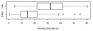
-Which season has the larger inter-quartile range (IQR) of monthly snowfall?
A) Early
B) Late
C) The two inter-quartile ranges are approximately equal.
D) The plot does not provide enough information to determine which inter-quartile range is larger.
-Which season has the larger inter-quartile range (IQR) of monthly snowfall?
A) Early
B) Late
C) The two inter-quartile ranges are approximately equal.
D) The plot does not provide enough information to determine which inter-quartile range is larger.
Question
Monthly snowfall (in inches) was measured over several winters in Fort Collins, Colorado. Researchers also recorded whether the measurement was taken in the Early winter (September to December) or Late winter (January to June). Boxplots displaying the distribution of monthly snowfall for each season are below.
-Which season has the larger median monthly snowfall?
A) Early
B) Late
C) The two medians are approximately equal.
D) The plot does not provide enough information to determine which median is larger.
-Which season has the larger median monthly snowfall?
A) Early
B) Late
C) The two medians are approximately equal.
D) The plot does not provide enough information to determine which median is larger.
Question
Monthly snowfall (in inches) was measured over several winters in Fort Collins, Colorado. Researchers also recorded whether the measurement was taken in the Early winter (September to December) or Late winter (January to June). Boxplots displaying the distribution of monthly snowfall for each season are below.
-The shape of the distribution of monthly snowfall measurements for the Early season is
A) symmetric.
B) skewed right.
C) skewed left.
D) bimodal.
-The shape of the distribution of monthly snowfall measurements for the Early season is
A) symmetric.
B) skewed right.
C) skewed left.
D) bimodal.
Question
Monthly snowfall (in inches) was measured over several winters in Fort Collins, Colorado. Researchers also recorded whether the measurement was taken in the Early winter (September to December) or Late winter (January to June). Boxplots displaying the distribution of monthly snowfall for each season are below.
-For the Early season data, if the largest outlier (with a monthly snowfall of 55 inches) were removed from the data set, the sample mean would
A) increase.
B) decrease.
C) remain approximately the same.
D) There is not enough information given to determine how the sample mean would change if the outlier is removed.
Question
Monthly snowfall (in inches) was measured over several winters in Fort Collins, Colorado. Researchers also recorded whether the measurement was taken in the Early winter (September to December) or Late winter (January to June). Boxplots displaying the distribution of monthly snowfall for each season are below.
-What is the upper quartile (Q3) of the distribution of monthly snowfall measurements for the Late season (approximately)?
A) 5
B) 22
C) 33
D) 41
E) 60
-What is the upper quartile (Q3) of the distribution of monthly snowfall measurements for the Late season (approximately)?
A) 5
B) 22
C) 33
D) 41
E) 60
Question
Monthly snowfall (in inches) was measured over several winters in Fort Collins, Colorado. Researchers also recorded whether the measurement was taken in the Early winter (September to December) or Late winter (January to June). Boxplots displaying the distribution of monthly snowfall for each season are below.
-Which of the following sentences correctly interprets the first quartile (Q1) of the distribution of monthly snowfall measurements for the Early season?
A) About 25% of Early season winter months in Fort Collins get less than 9 inches of snow.
B) About 50% of Early season winter months in Fort Collins get less than 9 inches of snow.
C) About 75% of Early season winter months in Fort Collins get less than 9 inches of snow.
D) About 25% of Early season winter months in Fort Collins get more than 38 inches of snow.
Question
Monthly snowfall (in inches) was measured over several winters in Fort Collins, Colorado. Researchers also recorded whether the measurement was taken in the Early winter (September to December) or Late winter (January to June). Boxplots displaying the distribution of monthly snowfall for each season are below.
-The boxplots demonstrate that there is an association between which two variables?
A) Early and Late winter season
B) Snowfall and months
C) Monthly snowfall and whether it was Early or Late winter season
D) Whether it was Early or Late winter season and months
-The boxplots demonstrate that there is an association between which two variables?
A) Early and Late winter season
B) Snowfall and months
C) Monthly snowfall and whether it was Early or Late winter season
D) Whether it was Early or Late winter season and months
Question
Question
Question
The plot below displays the on-base percentage for all Major League Baseball players who played in at least 15 games during the 2018 MLB season based on the player's position.
Positions: 1/2/3B = 1st/2nd/3rd base, C = catcher, C/L/RF = center/left/right field, DH = designated hitter, P = pitcher, SS = short stop
On-base percentage = (hits + walks + hit by pitch)/(total plate appearances)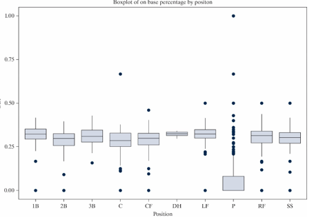
-Which of the positions has the smallest inter-quartile range (IQR) of on-base percentages?
A) 3B
B) CF
C) DH
D) P
Question
The plot below displays the on-base percentage for all Major League Baseball players who played in at least 15 games during the 2018 MLB season based on the player's position.
Positions: 1/2/3B = 1st/2nd/3rd base, C = catcher, C/L/RF = center/left/right field, DH = designated hitter, P = pitcher, SS = short stop
On-base percentage = (hits + walks + hit by pitch)/(total plate appearances)
-At least 50% of on-base percentages for the pitcher (P) are zero.
Positions: 1/2/3B = 1st/2nd/3rd base, C = catcher, C/L/RF = center/left/right field, DH = designated hitter, P = pitcher, SS = short stop
On-base percentage = (hits + walks + hit by pitch)/(total plate appearances)
-At least 50% of on-base percentages for the pitcher (P) are zero.
Question
The boxplots below display the distribution of maximum speed by type of roller coaster for a data set of 145 roller coasters in the United States. 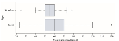
-For steel roller coasters, the interquartile range (IQR) is equal to
A) 10 mph.
B) 20 mph.
C) 70 mph.
D) 95 mph.
-For steel roller coasters, the interquartile range (IQR) is equal to
A) 10 mph.
B) 20 mph.
C) 70 mph.
D) 95 mph.
Question
The boxplots below display the distribution of maximum speed by type of roller coaster for a data set of 145 roller coasters in the United States.
-For steel roller coasters, if the outlier at 120 was removed, the sample mean would
A) increase.
B) decrease.
C) stay the same.
D) There is not enough information given to know if the sample mean would change.
-For steel roller coasters, if the outlier at 120 was removed, the sample mean would
A) increase.
B) decrease.
C) stay the same.
D) There is not enough information given to know if the sample mean would change.
Question
The boxplots below display the distribution of maximum speed by type of roller coaster for a data set of 145 roller coasters in the United States.
-The boxplots show that 25% of wooden roller coasters in the sample travel faster than
A) 50 mph.
B) 54 mph.
C) 60 mph
D) 65 mph.
-The boxplots show that 25% of wooden roller coasters in the sample travel faster than
A) 50 mph.
B) 54 mph.
C) 60 mph
D) 65 mph.
Question
The boxplots below display the distribution of maximum speed by type of roller coaster for a data set of 145 roller coasters in the United States.
-Which type of roller coaster has the larger median speed?
A) Steel
B) Wooden
C) The two types of roller coasters have the same median speed.
D) The plot does not provide enough information to determine which median is larger.
-Which type of roller coaster has the larger median speed?
A) Steel
B) Wooden
C) The two types of roller coasters have the same median speed.
D) The plot does not provide enough information to determine which median is larger.
Question
Do children diagnosed with attention deficit/hyperactivity disorder (ADHD) have smaller brains than children without this condition? Brain scans were completed for 152 children with ADHD and 139 children of similar age without ADHD. The mean brain size for the 152 children with ADHD was 1059.4 mL with a standard deviation of 117.5 mL. The mean brain size for the 139 children of with-out ADHD was 1104.5 mL with a standard deviation of 111.3 mL.
-State the appropriate null and alternative hypotheses for this research question, where 1 = ADHD and 2 = Without ADHD.
A) versus
B) versus
C) versus
D) versus
E) versus
  F.
F.  versus
-State the appropriate null and alternative hypotheses for this research question, where 1 = ADHD and 2 = Without ADHD.
A)
versus B)
versus C)
versus D)
versus E)
versus F. versus Question
Question
Question
Question
Question
Question
Question
What would the appropriate hypotheses be in order to investigate whether college upperclassmen tend to spend less on textbooks than college underclassmen?
A) versus
B)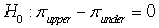 versus
C) versus
D)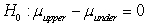 versus
A)
versus B)
versus C)
versus D)
versus Question
An article that appeared in the British Medical Journal (2010) presented the results of a randomized experiment conducted by researcher Jeremy Groves, whose objective was to determine whether the weight of his bicycle could affect his travel time to work. On each of 56 days (from mid-January to mid-July 2010), Groves tossed a £1 coin to decide whether he would be biking to work on his carbon frame (lighter) bicycle that weighed 20.9 lbs or on his steel frame (heavier) bicycle that weighed 29.75 lbs. He then recorded the commute time (in minutes) for each trip.
Here are the summary statistics for his data:
-In terms of investigating whether the lighter carbon frame bike will tend to have a higher or lower mean commute time compared to the heavier steel frame bike, which of the following is the correct null hypothesis?
A) There is an association between the type of bike frame and commute time.
B) There is no association between the type of bike frame and commute time.
C) There is an association between days and weight of bicycle.
D) There is no association between days and weight of bicycle.
Question
An article that appeared in the British Medical Journal (2010) presented the results of a randomized experiment conducted by researcher Jeremy Groves, whose objective was to determine whether the weight of his bicycle could affect his travel time to work. On each of 56 days (from mid-January to mid-July 2010), Groves tossed a £1 coin to decide whether he would be biking to work on his carbon frame (lighter) bicycle that weighed 20.9 lbs or on his steel frame (heavier) bicycle that weighed 29.75 lbs. He then recorded the commute time (in minutes) for each trip.
Here are the summary statistics for his data:
-In terms of investigating whether the lighter carbon frame bike will tend to have a higher or lower mean commute time compared to the heavier steel frame bike, which of the following is the correct alternative hypothesis?
A) There is an association between the type of bike frame and commute time.
B) There is no association between the type of bike frame and commute time.
C) There is an association between days and weight of bicycle.
D) There is no association between days and weight of bicycle.
Question
An article that appeared in the British Medical Journal (2010) presented the results of a randomized experiment conducted by researcher Jeremy Groves, whose objective was to determine whether the weight of his bicycle could affect his travel time to work. On each of 56 days (from mid-January to mid-July 2010), Groves tossed a £1 coin to decide whether he would be biking to work on his carbon frame (lighter) bicycle that weighed 20.9 lbs or on his steel frame (heavier) bicycle that weighed 29.75 lbs. He then recorded the commute time (in minutes) for each trip.
Here are the summary statistics for his data:
-Which of the following applets would be most appropriate to use, in the context of this study?
A) One Proportion
B) One Mean
C) Multiple Proportions
D) Multiple Means
E) Matched Pairs
Here are the summary statistics for his data:
-Which of the following applets would be most appropriate to use, in the context of this study?
A) One Proportion
B) One Mean
C) Multiple Proportions
D) Multiple Means
E) Matched Pairs
Question
An article that appeared in the British Medical Journal (2010) presented the results of a randomized experiment conducted by researcher Jeremy Groves, whose objective was to determine whether the weight of his bicycle could affect his travel time to work. On each of 56 days (from mid-January to mid-July 2010), Groves tossed a £1 coin to decide whether he would be biking to work on his carbon frame (lighter) bicycle that weighed 20.9 lbs or on his steel frame (heavier) bicycle that weighed 29.75 lbs. He then recorded the commute time (in minutes) for each trip.
Here are the summary statistics for his data:
-A 95% confidence interval for the difference in long-run mean commute time between frames (Carbon - Steel) is (-2.39, 3.45) min. How would you interpret this interval?
A) We are 95% confident that commute times are, on average, between 2.39 min faster to 3.45 min slower for carbon frames compared to steel frames.
B) We are 95% confident that commute times are, on average, between 2.39 min slower to 3.45 min faster for carbon frames compared to steel frames.
C) In 95% of all commutes, the carbon frame will be between 2.39 min faster to 3.45 min slower than the steel frame.
D) In 95% of all commutes, the carbon frame will be between 2.39 min slower to 3.45 min faster than the steel frame.
Question
An article that appeared in the British Medical Journal (2010) presented the results of a randomized experiment conducted by researcher Jeremy Groves, whose objective was to determine whether the weight of his bicycle could affect his travel time to work. On each of 56 days (from mid-January to mid-July 2010), Groves tossed a £1 coin to decide whether he would be biking to work on his carbon frame (lighter) bicycle that weighed 20.9 lbs or on his steel frame (heavier) bicycle that weighed 29.75 lbs. He then recorded the commute time (in minutes) for each trip.
Here are the summary statistics for his data:
-The p-value comparing the two average commute times for the two different bikes was found to be 0.728. Which of the following is the most appropriate conclusion based on this p-value?
A) There is evidence that the mean commute times for the two bike types are different.
B) There is evidence that the mean commute times for the two bike types are not different.
C) There is no evidence that the mean commute times for the two bike types are different.
D) None of the above.
Question
Question
Question
Question
An article that appeared in the British Medical Journal (2010) presented the results of a randomized experiment conducted by researcher Jeremy Groves, whose objective was to determine whether the weight of his bicycle could affect his travel time to work. On each of 56 days (from mid-January to mid-July 2010), Groves tossed a £1 coin to decide whether he would be biking to work on his carbon frame (lighter) bicycle that weighed 20.9 lbs or on his steel frame (heavier) bicycle that weighed 29.75 lbs. He then recorded the commute time (in minutes) for each trip.
Here are the summary statistics for his data: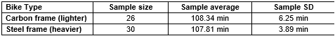
-Assuming the distribution of commute times is not strongly skewed in either sample, in evaluating the relationship between bike type and commute time, would a theory-based approach be valid?
A) Yes, since 56 is larger than 20.
B) Yes, since both 26 and 30 are larger than 20.
C) Yes, since both 26 and 30 are larger than 10.
D) No, a theory-based approach would not be valid.
Question
An article that appeared in the British Medical Journal (2010) presented the results of a randomized experiment conducted by researcher Jeremy Groves, whose objective was to determine whether the weight of his bicycle could affect his travel time to work. On each of 56 days (from mid-January to mid-July 2010), Groves tossed a £1 coin to decide whether he would be biking to work on his carbon frame (lighter) bicycle that weighed 20.9 lbs or on his steel frame (heavier) bicycle that weighed 29.75 lbs. He then recorded the commute time (in minutes) for each trip.
Here are the summary statistics for his data:
-Use the
Theory-Based Inference applet to find the theory-based p-value for the appropriate test of two means.
Here are the summary statistics for his data:
-Use the
Theory-Based Inference applet to find the theory-based p-value for the appropriate test of two means.
Question
An article that appeared in the British Medical Journal (2010) presented the results of a randomized experiment conducted by researcher Jeremy Groves, whose objective was to determine whether the weight of his bicycle could affect his travel time to work. On each of 56 days (from mid-January to mid-July 2010), Groves tossed a £1 coin to decide whether he would be biking to work on his carbon frame (lighter) bicycle that weighed 20.9 lbs or on his steel frame (heavier) bicycle that weighed 29.75 lbs. He then recorded the commute time (in minutes) for each trip.
Here are the summary statistics for his data:
-Calculate the standardized statistic for the appropriate test of two means (carbon - steel).
A) 0.71
B) 0.53
C) 0.37
D) 1.42
Here are the summary statistics for his data:
-Calculate the standardized statistic for the appropriate test of two means (carbon - steel).
A) 0.71
B) 0.53
C) 0.37
D) 1.42
Question
An article that appeared in the British Medical Journal (2010) presented the results of a randomized experiment conducted by researcher Jeremy Groves, whose objective was to determine whether the weight of his bicycle could affect his travel time to work. On each of 56 days (from mid-January to mid-July 2010), Groves tossed a £1 coin to decide whether he would be biking to work on his carbon frame (lighter) bicycle that weighed 20.9 lbs or on his steel frame (heavier) bicycle that weighed 29.75 lbs. He then recorded the commute time (in minutes) for each trip.
Here are the summary statistics for his data:
-Under the null hypothesis, what distribution does the test statistic follow?
A) Standard normal distribution
B) t-distribution
C) Skewed distribution
D) Normal distribution
Here are the summary statistics for his data:
-Under the null hypothesis, what distribution does the test statistic follow?
A) Standard normal distribution
B) t-distribution
C) Skewed distribution
D) Normal distribution
Question
Question
Question
Question
Question
In order to investigate whether talking on cell phones is more distracting than listening to car radios while driving, sixty-four student volunteers (from a single college class) were randomly assigned to a cell phone group or a radio group (32 students were assigned to each group). Each student "drove" a machine that simulated driving situations. While "driving" the simulator, a target would flash red at irregular intervals. Participants were instructed to press the "brake" button as soon as possible when they detected a red light. Participant response times were measured as the time between the red light appearing and pushing the brake button. While driving, the radio group listened to a radio broadcast and the cell phone group carried on a conversation on the cell phone with someone in the next room.
The cell phone group had an average response time of 585.2 milliseconds (SD = 89.6), and the control group had an average response time of 533.7 milliseconds (SD = 65.3).
-Use the
Theory-Based Inference applet to find the theory-based 99% confidence interval for .
 (___(1)___, ___(2)___)
The cell phone group had an average response time of 585.2 milliseconds (SD = 89.6), and the control group had an average response time of 533.7 milliseconds (SD = 65.3).
-Use the
Theory-Based Inference applet to find the theory-based 99% confidence interval for .
(___(1)___, ___(2)___) Question
Question
A random sample of Hope College students was taken and one of the questions asked was how many hours per week they study. You want to see if there is a difference between males and females in terms of average study time. The sample results are given in the following table. 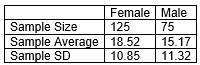
-Assuming the distribution of study times is not strongly skewed for either sample, which approach would be more appropriate for these data: simulation-based or theory-based?
A) Simulation-based, since this approach works for any sample size.
B) Theory-based, since both 125 and 75 are greater than 20.
C) Either approach would be appropriate.
D) Neither approach would be appropriate.
Question
A random sample of Hope College students was taken and one of the questions asked was how many hours per week they study. You want to see if there is a difference between males and females in terms of average study time. The sample results are given in the following table.
-Which "Scenario" would you choose from the pull-down menu of the Theory-Based Inference applet?
A) One proportion
B) One mean
C) Two proportions
D) Two means
-Which "Scenario" would you choose from the pull-down menu of the Theory-Based Inference applet?
A) One proportion
B) One mean
C) Two proportions
D) Two means
Question
When newborns are held so that their feet just barely touch the floor, they will make instinctive walking and placing motions. This reflex disappears by about eight weeks. Researchers wanted to know if stimulating this behavior in infants during their first eight weeks of life would lead them to walk at an earlier age compared to infants who do not receive this stimulation. To test this they had twelve infants randomly assigned to two groups. Six infants received stimulation of the walking and placing reflex (active group) and six infants receive equal amounts of gross motor and social stimulation, but did not received stimulation of the walking and placing reflex (passive group). The researchers then compared the infant's age (in months) when they first walked and the results are shown in the following figure. 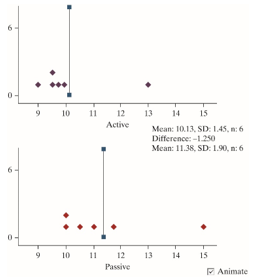
-State the null and alternative hypotheses for this research question, where 1 = Active and 2 = Passive.
A) versus
B) versus
C) versus
D) versus
E) versus
F) versus
-State the null and alternative hypotheses for this research question, where 1 = Active and 2 = Passive.
A)
versus B)
versus C)
versus D)
versus E)
versus F)
versus Question
When newborns are held so that their feet just barely touch the floor, they will make instinctive walking and placing motions. This reflex disappears by about eight weeks. Researchers wanted to know if stimulating this behavior in infants during their first eight weeks of life would lead them to walk at an earlier age compared to infants who do not receive this stimulation. To test this they had twelve infants randomly assigned to two groups. Six infants received stimulation of the walking and placing reflex (active group) and six infants receive equal amounts of gross motor and social stimulation, but did not received stimulation of the walking and placing reflex (passive group). The researchers then compared the infant's age (in months) when they first walked and the results are shown in the following figure.
-In evaluating the relationship between whether an infant received stimulation of the walking and placing reflex and the infant's age when they first walked, would a theory-based approach be valid?
A) Yes, since 12 is larger than 10.
B) No, since 6 and 6 are both less than 20 and each sample has an outlier.
C) Yes, since we are testing a difference in means.
D) No, since the researchers did not use a random sample.
Question
When newborns are held so that their feet just barely touch the floor, they will make instinctive walking and placing motions. This reflex disappears by about eight weeks. Researchers wanted to know if stimulating this behavior in infants during their first eight weeks of life would lead them to walk at an earlier age compared to infants who do not receive this stimulation. To test this they had twelve infants randomly assigned to two groups. Six infants received stimulation of the walking and placing reflex (active group) and six infants receive equal amounts of gross motor and social stimulation, but did not received stimulation of the walking and placing reflex (passive group). The researchers then compared the infant's age (in months) when they first walked and the results are shown in the following figure.
-Which of the following applets would be most appropriate to use, in the context of this study?
A) One Proportion
B) One Mean
C) Multiple Proportions
D) Multiple Means
E) Matched Pairs F. Theory-Based Inference
-Which of the following applets would be most appropriate to use, in the context of this study?
A) One Proportion
B) One Mean
C) Multiple Proportions
D) Multiple Means
E) Matched Pairs F. Theory-Based Inference

Unlock Deck
Sign up to unlock the cards in this deck!
Unlock Deck
Unlock Deck
1/46
Play
Full screen (f)
Deck 7: Comparing Two Means
1
Monthly snowfall (in inches) was measured over several winters in Fort Collins, Colorado. Researchers also recorded whether the measurement was taken in the Early winter (September to December) or Late winter (January to June). Boxplots displaying the distribution of monthly snowfall for each season are below.
-Which season has the larger inter-quartile range (IQR) of monthly snowfall?
A) Early
B) Late
C) The two inter-quartile ranges are approximately equal.
D) The plot does not provide enough information to determine which inter-quartile range is larger.
-Which season has the larger inter-quartile range (IQR) of monthly snowfall?
A) Early
B) Late
C) The two inter-quartile ranges are approximately equal.
D) The plot does not provide enough information to determine which inter-quartile range is larger.
Late
2
Monthly snowfall (in inches) was measured over several winters in Fort Collins, Colorado. Researchers also recorded whether the measurement was taken in the Early winter (September to December) or Late winter (January to June). Boxplots displaying the distribution of monthly snowfall for each season are below.
-Which season has the larger median monthly snowfall?
A) Early
B) Late
C) The two medians are approximately equal.
D) The plot does not provide enough information to determine which median is larger.
-Which season has the larger median monthly snowfall?
A) Early
B) Late
C) The two medians are approximately equal.
D) The plot does not provide enough information to determine which median is larger.
Late
3
Monthly snowfall (in inches) was measured over several winters in Fort Collins, Colorado. Researchers also recorded whether the measurement was taken in the Early winter (September to December) or Late winter (January to June). Boxplots displaying the distribution of monthly snowfall for each season are below.
-The shape of the distribution of monthly snowfall measurements for the Early season is
A) symmetric.
B) skewed right.
C) skewed left.
D) bimodal.
-The shape of the distribution of monthly snowfall measurements for the Early season is
A) symmetric.
B) skewed right.
C) skewed left.
D) bimodal.
skewed left.
4
Monthly snowfall (in inches) was measured over several winters in Fort Collins, Colorado. Researchers also recorded whether the measurement was taken in the Early winter (September to December) or Late winter (January to June). Boxplots displaying the distribution of monthly snowfall for each season are below.
-For the Early season data, if the largest outlier (with a monthly snowfall of 55 inches) were removed from the data set, the sample mean would
A) increase.
B) decrease.
C) remain approximately the same.
D) There is not enough information given to determine how the sample mean would change if the outlier is removed.
Unlock Deck
Unlock for access to all 46 flashcards in this deck.
Unlock Deck
k this deck
5
Monthly snowfall (in inches) was measured over several winters in Fort Collins, Colorado. Researchers also recorded whether the measurement was taken in the Early winter (September to December) or Late winter (January to June). Boxplots displaying the distribution of monthly snowfall for each season are below.
-What is the upper quartile (Q3) of the distribution of monthly snowfall measurements for the Late season (approximately)?
A) 5
B) 22
C) 33
D) 41
E) 60
-What is the upper quartile (Q3) of the distribution of monthly snowfall measurements for the Late season (approximately)?
A) 5
B) 22
C) 33
D) 41
E) 60
Unlock Deck
Unlock for access to all 46 flashcards in this deck.
Unlock Deck
k this deck
6
Monthly snowfall (in inches) was measured over several winters in Fort Collins, Colorado. Researchers also recorded whether the measurement was taken in the Early winter (September to December) or Late winter (January to June). Boxplots displaying the distribution of monthly snowfall for each season are below.
-Which of the following sentences correctly interprets the first quartile (Q1) of the distribution of monthly snowfall measurements for the Early season?
A) About 25% of Early season winter months in Fort Collins get less than 9 inches of snow.
B) About 50% of Early season winter months in Fort Collins get less than 9 inches of snow.
C) About 75% of Early season winter months in Fort Collins get less than 9 inches of snow.
D) About 25% of Early season winter months in Fort Collins get more than 38 inches of snow.
Unlock Deck
Unlock for access to all 46 flashcards in this deck.
Unlock Deck
k this deck
7
Monthly snowfall (in inches) was measured over several winters in Fort Collins, Colorado. Researchers also recorded whether the measurement was taken in the Early winter (September to December) or Late winter (January to June). Boxplots displaying the distribution of monthly snowfall for each season are below.
-The boxplots demonstrate that there is an association between which two variables?
A) Early and Late winter season
B) Snowfall and months
C) Monthly snowfall and whether it was Early or Late winter season
D) Whether it was Early or Late winter season and months
-The boxplots demonstrate that there is an association between which two variables?
A) Early and Late winter season
B) Snowfall and months
C) Monthly snowfall and whether it was Early or Late winter season
D) Whether it was Early or Late winter season and months
Unlock Deck
Unlock for access to all 46 flashcards in this deck.
Unlock Deck
k this deck
8
Which of the following plots is not appropriate for a quantitative variable?
A) Bar graph
B) Dot plot
C) Histogram
D) Boxplot
A) Bar graph
B) Dot plot
C) Histogram
D) Boxplot
Unlock Deck
Unlock for access to all 46 flashcards in this deck.
Unlock Deck
k this deck
9
Which of the following data sets has the largest standard deviation?
A) 1, 2, 3, 4, 5
B) 1, 3, 3, 3, 5
C) 1, 1, 3, 5, 5
D) 1, 1, 1, 1, 1
A) 1, 2, 3, 4, 5
B) 1, 3, 3, 3, 5
C) 1, 1, 3, 5, 5
D) 1, 1, 1, 1, 1
Unlock Deck
Unlock for access to all 46 flashcards in this deck.
Unlock Deck
k this deck
10
The plot below displays the on-base percentage for all Major League Baseball players who played in at least 15 games during the 2018 MLB season based on the player's position.
Positions: 1/2/3B = 1st/2nd/3rd base, C = catcher, C/L/RF = center/left/right field, DH = designated hitter, P = pitcher, SS = short stop
On-base percentage = (hits + walks + hit by pitch)/(total plate appearances)
-Which of the positions has the smallest inter-quartile range (IQR) of on-base percentages?
A) 3B
B) CF
C) DH
D) P
Unlock Deck
Unlock for access to all 46 flashcards in this deck.
Unlock Deck
k this deck
11
The plot below displays the on-base percentage for all Major League Baseball players who played in at least 15 games during the 2018 MLB season based on the player's position.
Positions: 1/2/3B = 1st/2nd/3rd base, C = catcher, C/L/RF = center/left/right field, DH = designated hitter, P = pitcher, SS = short stop
On-base percentage = (hits + walks + hit by pitch)/(total plate appearances)
-At least 50% of on-base percentages for the pitcher (P) are zero.
Positions: 1/2/3B = 1st/2nd/3rd base, C = catcher, C/L/RF = center/left/right field, DH = designated hitter, P = pitcher, SS = short stop
On-base percentage = (hits + walks + hit by pitch)/(total plate appearances)
-At least 50% of on-base percentages for the pitcher (P) are zero.
Unlock Deck
Unlock for access to all 46 flashcards in this deck.
Unlock Deck
k this deck
12
The boxplots below display the distribution of maximum speed by type of roller coaster for a data set of 145 roller coasters in the United States.
-For steel roller coasters, the interquartile range (IQR) is equal to
A) 10 mph.
B) 20 mph.
C) 70 mph.
D) 95 mph.
-For steel roller coasters, the interquartile range (IQR) is equal to
A) 10 mph.
B) 20 mph.
C) 70 mph.
D) 95 mph.
Unlock Deck
Unlock for access to all 46 flashcards in this deck.
Unlock Deck
k this deck
13
The boxplots below display the distribution of maximum speed by type of roller coaster for a data set of 145 roller coasters in the United States.
-For steel roller coasters, if the outlier at 120 was removed, the sample mean would
A) increase.
B) decrease.
C) stay the same.
D) There is not enough information given to know if the sample mean would change.
-For steel roller coasters, if the outlier at 120 was removed, the sample mean would
A) increase.
B) decrease.
C) stay the same.
D) There is not enough information given to know if the sample mean would change.
Unlock Deck
Unlock for access to all 46 flashcards in this deck.
Unlock Deck
k this deck
14
The boxplots below display the distribution of maximum speed by type of roller coaster for a data set of 145 roller coasters in the United States.
-The boxplots show that 25% of wooden roller coasters in the sample travel faster than
A) 50 mph.
B) 54 mph.
C) 60 mph
D) 65 mph.
-The boxplots show that 25% of wooden roller coasters in the sample travel faster than
A) 50 mph.
B) 54 mph.
C) 60 mph
D) 65 mph.
Unlock Deck
Unlock for access to all 46 flashcards in this deck.
Unlock Deck
k this deck
15
The boxplots below display the distribution of maximum speed by type of roller coaster for a data set of 145 roller coasters in the United States.
-Which type of roller coaster has the larger median speed?
A) Steel
B) Wooden
C) The two types of roller coasters have the same median speed.
D) The plot does not provide enough information to determine which median is larger.
-Which type of roller coaster has the larger median speed?
A) Steel
B) Wooden
C) The two types of roller coasters have the same median speed.
D) The plot does not provide enough information to determine which median is larger.
Unlock Deck
Unlock for access to all 46 flashcards in this deck.
Unlock Deck
k this deck
16
Do children diagnosed with attention deficit/hyperactivity disorder (ADHD) have smaller brains than children without this condition? Brain scans were completed for 152 children with ADHD and 139 children of similar age without ADHD. The mean brain size for the 152 children with ADHD was 1059.4 mL with a standard deviation of 117.5 mL. The mean brain size for the 139 children of with-out ADHD was 1104.5 mL with a standard deviation of 111.3 mL.
-State the appropriate null and alternative hypotheses for this research question, where 1 = ADHD and 2 = Without ADHD.
A) versus
B) versus
C) versus
D) versus
E) versus F. versus
-State the appropriate null and alternative hypotheses for this research question, where 1 = ADHD and 2 = Without ADHD.
A)
versus B)
versus C)
versus D)
versus E)
versus F. versus Unlock Deck
Unlock for access to all 46 flashcards in this deck.
Unlock Deck
k this deck
17
Do children diagnosed with attention deficit/hyperactivity disorder (ADHD) have smaller brains than children without this condition? Brain scans were completed for 152 children with ADHD and 139 children of similar age without ADHD. The mean brain size for the 152 children with ADHD was 1059.4 mL with a standard deviation of 117.5 mL. The mean brain size for the 139 children of with-out ADHD was 1104.5 mL with a standard deviation of 111.3 mL.
-What is the value of the statistic we should use in the 3S strategy?
A) 1059.4
B) 1104.5
C) -45.1
D) 6.2
-What is the value of the statistic we should use in the 3S strategy?
A) 1059.4
B) 1104.5
C) -45.1
D) 6.2
Unlock Deck
Unlock for access to all 46 flashcards in this deck.
Unlock Deck
k this deck
18
Do children diagnosed with attention deficit/hyperactivity disorder (ADHD) have smaller brains than children without this condition? Brain scans were completed for 152 children with ADHD and 139 children of similar age without ADHD. The mean brain size for the 152 children with ADHD was 1059.4 mL with a standard deviation of 117.5 mL. The mean brain size for the 139 children of with-out ADHD was 1104.5 mL with a standard deviation of 111.3 mL.
-How could you simulate one sample under the null hypothesis?
A) Take 152 red cards and 139 blue cards, shuffle the cards and randomly deal them into two piles of size 152 and 139. Calculate the difference in proportion of red cards between the two samples.
B) Write the children's ages on 291 cards, shuffle the cards and randomly deal them into two piles of size 152 and 139. Calculate the difference in mean age between the two samples.
C) Write the children's brain sizes on 291 cards, shuffle the cards and randomly deal them into two piles of size 152 and 139. Calculate the difference in mean brain size between the two samples.
D) Write the children's brain sizes on 291 cards, shuffle the cards and randomly deal them into two piles of size 152 and 139. Calculate the difference in standard deviation of brain size between the two samples.
Unlock Deck
Unlock for access to all 46 flashcards in this deck.
Unlock Deck
k this deck
19
Do children diagnosed with attention deficit/hyperactivity disorder (ADHD) have smaller brains than children without this condition? Brain scans were completed for 152 children with ADHD and 139 children of similar age without ADHD. The mean brain size for the 152 children with ADHD was 1059.4 mL with a standard deviation of 117.5 mL. The mean brain size for the 139 children of with-out ADHD was 1104.5 mL with a standard deviation of 111.3 mL.
-The standard deviation of a simulated null distribution of 1,000 differences in sample mean brain sizes was 13.4 mL. Calculate the standardized statistic for a test of two means (ADHD - Without ADHD).
-The standard deviation of a simulated null distribution of 1,000 differences in sample mean brain sizes was 13.4 mL. Calculate the standardized statistic for a test of two means (ADHD - Without ADHD).
Unlock Deck
Unlock for access to all 46 flashcards in this deck.
Unlock Deck
k this deck
20
Do children diagnosed with attention deficit/hyperactivity disorder (ADHD) have smaller brains than children without this condition? Brain scans were completed for 152 children with ADHD and 139 children of similar age without ADHD. The mean brain size for the 152 children with ADHD was 1059.4 mL with a standard deviation of 117.5 mL. The mean brain size for the 139 children of with-out ADHD was 1104.5 mL with a standard deviation of 111.3 mL.
-The standard deviation of a simulated null distribution of 1,000 differences in sample mean brain sizes was 13.4 mL. Use the 2SD method to calculate an approximate 95% confidence interval for the difference in population means (ADHD - Without ADHD).
(___(1)___, ___(2)___)
-The standard deviation of a simulated null distribution of 1,000 differences in sample mean brain sizes was 13.4 mL. Use the 2SD method to calculate an approximate 95% confidence interval for the difference in population means (ADHD - Without ADHD).
(___(1)___, ___(2)___)
Unlock Deck
Unlock for access to all 46 flashcards in this deck.
Unlock Deck
k this deck
21
Do children diagnosed with attention deficit/hyperactivity disorder (ADHD) have smaller brains than children without this condition? Brain scans were completed for 152 children with ADHD and 139 children of similar age without ADHD. The mean brain size for the 152 children with ADHD was 1059.4 mL with a standard deviation of 117.5 mL. The mean brain size for the 139 children of with-out ADHD was 1104.5 mL with a standard deviation of 111.3 mL.
-The p-value from a simulation-based hypothesis test for these data is 0.0003. What conclusion can be made based upon this p-value?
A) We have strong evidence that ADHD leads to smaller brain sizes among children similar to those in the study.
B) We have strong evidence that ADHD leads to smaller brain sizes among all children.
C) We have strong evidence that ADHD is associated with smaller brain sizes among children similar to those in the study.
D) We have strong evidence that ADHD is associated with smaller brain sizes among all children.
Unlock Deck
Unlock for access to all 46 flashcards in this deck.
Unlock Deck
k this deck
22
A researcher asked random samples of 50 kindergarten teachers and 50 12th grade teachers how much money they spent out-of-pocket on school supplies in the previous school year,
To see if teachers at one grade level spent more than the other. A 95% confidence interval for ?K ? ?12 is $30 to $50. Based on this result, it is reasonable to conclude that
A) 95% of all kindergarten teachers spend between $30 and $50 more than 95% of all 12th grade teachers.
B) each kindergarten teacher spends $30 to $50 more than any 12th grade teacher.
C) kindergarten teachers spend more on average than do 12th grade teachers.
D) 12th grade teachers spend more on average than do kindergarten teachers.
Unlock Deck
Unlock for access to all 46 flashcards in this deck.
Unlock Deck
k this deck
23
What would the appropriate hypotheses be in order to investigate whether college upperclassmen tend to spend less on textbooks than college underclassmen?
A) versus
B) versus
C) versus
D) versus
A)
versus B)
versus C)
versus D)
versus Unlock Deck
Unlock for access to all 46 flashcards in this deck.
Unlock Deck
k this deck
24
An article that appeared in the British Medical Journal (2010) presented the results of a randomized experiment conducted by researcher Jeremy Groves, whose objective was to determine whether the weight of his bicycle could affect his travel time to work. On each of 56 days (from mid-January to mid-July 2010), Groves tossed a £1 coin to decide whether he would be biking to work on his carbon frame (lighter) bicycle that weighed 20.9 lbs or on his steel frame (heavier) bicycle that weighed 29.75 lbs. He then recorded the commute time (in minutes) for each trip.
Here are the summary statistics for his data:
-In terms of investigating whether the lighter carbon frame bike will tend to have a higher or lower mean commute time compared to the heavier steel frame bike, which of the following is the correct null hypothesis?
A) There is an association between the type of bike frame and commute time.
B) There is no association between the type of bike frame and commute time.
C) There is an association between days and weight of bicycle.
D) There is no association between days and weight of bicycle.
Unlock Deck
Unlock for access to all 46 flashcards in this deck.
Unlock Deck
k this deck
25
An article that appeared in the British Medical Journal (2010) presented the results of a randomized experiment conducted by researcher Jeremy Groves, whose objective was to determine whether the weight of his bicycle could affect his travel time to work. On each of 56 days (from mid-January to mid-July 2010), Groves tossed a £1 coin to decide whether he would be biking to work on his carbon frame (lighter) bicycle that weighed 20.9 lbs or on his steel frame (heavier) bicycle that weighed 29.75 lbs. He then recorded the commute time (in minutes) for each trip.
Here are the summary statistics for his data:
-In terms of investigating whether the lighter carbon frame bike will tend to have a higher or lower mean commute time compared to the heavier steel frame bike, which of the following is the correct alternative hypothesis?
A) There is an association between the type of bike frame and commute time.
B) There is no association between the type of bike frame and commute time.
C) There is an association between days and weight of bicycle.
D) There is no association between days and weight of bicycle.
Unlock Deck
Unlock for access to all 46 flashcards in this deck.
Unlock Deck
k this deck
26
An article that appeared in the British Medical Journal (2010) presented the results of a randomized experiment conducted by researcher Jeremy Groves, whose objective was to determine whether the weight of his bicycle could affect his travel time to work. On each of 56 days (from mid-January to mid-July 2010), Groves tossed a £1 coin to decide whether he would be biking to work on his carbon frame (lighter) bicycle that weighed 20.9 lbs or on his steel frame (heavier) bicycle that weighed 29.75 lbs. He then recorded the commute time (in minutes) for each trip.
Here are the summary statistics for his data:
-Which of the following applets would be most appropriate to use, in the context of this study?
A) One Proportion
B) One Mean
C) Multiple Proportions
D) Multiple Means
E) Matched Pairs
Here are the summary statistics for his data:
-Which of the following applets would be most appropriate to use, in the context of this study?
A) One Proportion
B) One Mean
C) Multiple Proportions
D) Multiple Means
E) Matched Pairs
Unlock Deck
Unlock for access to all 46 flashcards in this deck.
Unlock Deck
k this deck
27
An article that appeared in the British Medical Journal (2010) presented the results of a randomized experiment conducted by researcher Jeremy Groves, whose objective was to determine whether the weight of his bicycle could affect his travel time to work. On each of 56 days (from mid-January to mid-July 2010), Groves tossed a £1 coin to decide whether he would be biking to work on his carbon frame (lighter) bicycle that weighed 20.9 lbs or on his steel frame (heavier) bicycle that weighed 29.75 lbs. He then recorded the commute time (in minutes) for each trip.
Here are the summary statistics for his data:
-A 95% confidence interval for the difference in long-run mean commute time between frames (Carbon - Steel) is (-2.39, 3.45) min. How would you interpret this interval?
A) We are 95% confident that commute times are, on average, between 2.39 min faster to 3.45 min slower for carbon frames compared to steel frames.
B) We are 95% confident that commute times are, on average, between 2.39 min slower to 3.45 min faster for carbon frames compared to steel frames.
C) In 95% of all commutes, the carbon frame will be between 2.39 min faster to 3.45 min slower than the steel frame.
D) In 95% of all commutes, the carbon frame will be between 2.39 min slower to 3.45 min faster than the steel frame.
Unlock Deck
Unlock for access to all 46 flashcards in this deck.
Unlock Deck
k this deck
28
An article that appeared in the British Medical Journal (2010) presented the results of a randomized experiment conducted by researcher Jeremy Groves, whose objective was to determine whether the weight of his bicycle could affect his travel time to work. On each of 56 days (from mid-January to mid-July 2010), Groves tossed a £1 coin to decide whether he would be biking to work on his carbon frame (lighter) bicycle that weighed 20.9 lbs or on his steel frame (heavier) bicycle that weighed 29.75 lbs. He then recorded the commute time (in minutes) for each trip.
Here are the summary statistics for his data:
-The p-value comparing the two average commute times for the two different bikes was found to be 0.728. Which of the following is the most appropriate conclusion based on this p-value?
A) There is evidence that the mean commute times for the two bike types are different.
B) There is evidence that the mean commute times for the two bike types are not different.
C) There is no evidence that the mean commute times for the two bike types are different.
D) None of the above.
Unlock Deck
Unlock for access to all 46 flashcards in this deck.
Unlock Deck
k this deck
29
In order to investigate whether talking on cell phones is more distracting than listening to car radios while driving, sixty-four student volunteers (from a single college class) were randomly assigned to a cell phone group or a radio group (32 students were assigned to each group). Each student "drove" a machine that simulated driving situations. While "driving" the simulator, a target would flash red at irregular intervals. Participants were instructed to press the "brake" button as soon as possible when they detected a red light. Participant response times were measured as the time between the red light appearing and pushing the brake button. While driving, the radio group listened to a radio broadcast and the cell phone group carried on a conversation on the cell phone with someone in the next room.
The cell phone group had an average response time of 585.2 milliseconds (SD = 89.6), and the control group had an average response time of 533.7 milliseconds (SD = 65.3).
-Which of the following applets would be most appropriate to use, in the context of this study?
A) One Proportion
B) One Mean
C) Multiple Proportions
D) Multiple Means
E) Matched Pairs
Unlock Deck
Unlock for access to all 46 flashcards in this deck.
Unlock Deck
k this deck
30
In order to investigate whether talking on cell phones is more distracting than listening to car radios while driving, sixty-four student volunteers (from a single college class) were randomly assigned to a cell phone group or a radio group (32 students were assigned to each group). Each student "drove" a machine that simulated driving situations. While "driving" the simulator, a target would flash red at irregular intervals. Participants were instructed to press the "brake" button as soon as possible when they detected a red light. Participant response times were measured as the time between the red light appearing and pushing the brake button. While driving, the radio group listened to a radio broadcast and the cell phone group carried on a conversation on the cell phone with someone in the next room.
The cell phone group had an average response time of 585.2 milliseconds (SD = 89.6), and the control group had an average response time of 533.7 milliseconds (SD = 65.3).
-Describe the parameter of interest in words.
A) Mean response time under simulated driving situations.
B) Difference in long-run mean response time between drivers talking on cell phones and drivers who listen to a radio broadcast.
C) Difference in long-run proportion of response times between drivers talking on cell phones and drivers who listen to a radio broadcast.
D) Difference in sample mean response time between drivers talking on cell phones and drivers who listen to a radio broadcast.
Unlock Deck
Unlock for access to all 46 flashcards in this deck.
Unlock Deck
k this deck
31
In order to investigate whether talking on cell phones is more distracting than listening to car radios while driving, sixty-four student volunteers (from a single college class) were randomly assigned to a cell phone group or a radio group (32 students were assigned to each group). Each student "drove" a machine that simulated driving situations. While "driving" the simulator, a target would flash red at irregular intervals. Participants were instructed to press the "brake" button as soon as possible when they detected a red light. Participant response times were measured as the time between the red light appearing and pushing the brake button. While driving, the radio group listened to a radio broadcast and the cell phone group carried on a conversation on the cell phone with someone in the next room.
The cell phone group had an average response time of 585.2 milliseconds (SD = 89.6), and the control group had an average response time of 533.7 milliseconds (SD = 65.3).
-Suppose you would like to use a simulation-based method to randomly shuffle the reaction times between the two groups. What would be the main purpose of this use of random shuffling in this simulation?
A) To allow cause-and-effect conclusions to be drawn from the study.
B) To allow generalizing the results to a larger population.
C) To simulate values of the statistic under the null hypothesis.
D) To replicate the study and increase the accuracy of the results.
Unlock Deck
Unlock for access to all 46 flashcards in this deck.
Unlock Deck
k this deck
32
An article that appeared in the British Medical Journal (2010) presented the results of a randomized experiment conducted by researcher Jeremy Groves, whose objective was to determine whether the weight of his bicycle could affect his travel time to work. On each of 56 days (from mid-January to mid-July 2010), Groves tossed a £1 coin to decide whether he would be biking to work on his carbon frame (lighter) bicycle that weighed 20.9 lbs or on his steel frame (heavier) bicycle that weighed 29.75 lbs. He then recorded the commute time (in minutes) for each trip.
Here are the summary statistics for his data:
-Assuming the distribution of commute times is not strongly skewed in either sample, in evaluating the relationship between bike type and commute time, would a theory-based approach be valid?
A) Yes, since 56 is larger than 20.
B) Yes, since both 26 and 30 are larger than 20.
C) Yes, since both 26 and 30 are larger than 10.
D) No, a theory-based approach would not be valid.
Unlock Deck
Unlock for access to all 46 flashcards in this deck.
Unlock Deck
k this deck
33
An article that appeared in the British Medical Journal (2010) presented the results of a randomized experiment conducted by researcher Jeremy Groves, whose objective was to determine whether the weight of his bicycle could affect his travel time to work. On each of 56 days (from mid-January to mid-July 2010), Groves tossed a £1 coin to decide whether he would be biking to work on his carbon frame (lighter) bicycle that weighed 20.9 lbs or on his steel frame (heavier) bicycle that weighed 29.75 lbs. He then recorded the commute time (in minutes) for each trip.
Here are the summary statistics for his data:
-Use the
Theory-Based Inference applet to find the theory-based p-value for the appropriate test of two means.
Here are the summary statistics for his data:
-Use the
Theory-Based Inference applet to find the theory-based p-value for the appropriate test of two means.
Unlock Deck
Unlock for access to all 46 flashcards in this deck.
Unlock Deck
k this deck
34
An article that appeared in the British Medical Journal (2010) presented the results of a randomized experiment conducted by researcher Jeremy Groves, whose objective was to determine whether the weight of his bicycle could affect his travel time to work. On each of 56 days (from mid-January to mid-July 2010), Groves tossed a £1 coin to decide whether he would be biking to work on his carbon frame (lighter) bicycle that weighed 20.9 lbs or on his steel frame (heavier) bicycle that weighed 29.75 lbs. He then recorded the commute time (in minutes) for each trip.
Here are the summary statistics for his data:
-Calculate the standardized statistic for the appropriate test of two means (carbon - steel).
A) 0.71
B) 0.53
C) 0.37
D) 1.42
Here are the summary statistics for his data:
-Calculate the standardized statistic for the appropriate test of two means (carbon - steel).
A) 0.71
B) 0.53
C) 0.37
D) 1.42
Unlock Deck
Unlock for access to all 46 flashcards in this deck.
Unlock Deck
k this deck
35
An article that appeared in the British Medical Journal (2010) presented the results of a randomized experiment conducted by researcher Jeremy Groves, whose objective was to determine whether the weight of his bicycle could affect his travel time to work. On each of 56 days (from mid-January to mid-July 2010), Groves tossed a £1 coin to decide whether he would be biking to work on his carbon frame (lighter) bicycle that weighed 20.9 lbs or on his steel frame (heavier) bicycle that weighed 29.75 lbs. He then recorded the commute time (in minutes) for each trip.
Here are the summary statistics for his data:
-Under the null hypothesis, what distribution does the test statistic follow?
A) Standard normal distribution
B) t-distribution
C) Skewed distribution
D) Normal distribution
Here are the summary statistics for his data:
-Under the null hypothesis, what distribution does the test statistic follow?
A) Standard normal distribution
B) t-distribution
C) Skewed distribution
D) Normal distribution
Unlock Deck
Unlock for access to all 46 flashcards in this deck.
Unlock Deck
k this deck
36
In order to investigate whether talking on cell phones is more distracting than listening to car radios while driving, sixty-four student volunteers (from a single college class) were randomly assigned to a cell phone group or a radio group (32 students were assigned to each group). Each student "drove" a machine that simulated driving situations. While "driving" the simulator, a target would flash red at irregular intervals. Participants were instructed to press the "brake" button as soon as possible when they detected a red light. Participant response times were measured as the time between the red light appearing and pushing the brake button. While driving, the radio group listened to a radio broadcast and the cell phone group carried on a conversation on the cell phone with someone in the next room.
The cell phone group had an average response time of 585.2 milliseconds (SD = 89.6), and the control group had an average response time of 533.7 milliseconds (SD = 65.3).
-In terms of investigating whether talking on cell phones is more distracting than listening to car radios while driving, which of the following is the correct null hypothesis?
A) There is an association between whether one talks on a cell phone or listens to the radio while driving and response time.
B) There is no association between whether one talks on a cell phone or listens to the radio while driving and response time.
C) Talking on a cell phone increases your response time compared to listening to the radio.
D) Talking on a cell phone does not increase your response time compared to listening to the radio.
Unlock Deck
Unlock for access to all 46 flashcards in this deck.
Unlock Deck
k this deck
37
In order to investigate whether talking on cell phones is more distracting than listening to car radios while driving, sixty-four student volunteers (from a single college class) were randomly assigned to a cell phone group or a radio group (32 students were assigned to each group). Each student "drove" a machine that simulated driving situations. While "driving" the simulator, a target would flash red at irregular intervals. Participants were instructed to press the "brake" button as soon as possible when they detected a red light. Participant response times were measured as the time between the red light appearing and pushing the brake button. While driving, the radio group listened to a radio broadcast and the cell phone group carried on a conversation on the cell phone with someone in the next room.
The cell phone group had an average response time of 585.2 milliseconds (SD = 89.6), and the control group had an average response time of 533.7 milliseconds (SD = 65.3).
-Assuming the distribution of response times is not strongly skewed in either sample, in evaluating the relationship between whether talking on a cell phone or listening to the radio and response time, would a theory-based approach be valid?
A) Yes, since 64 is larger than 20.
B) Yes, since 32 is larger than 20.
C) Yes, since both 585.2 and 533.7 are larger than 20.
D) No, a theory-based approach would not be valid.
Unlock Deck
Unlock for access to all 46 flashcards in this deck.
Unlock Deck
k this deck
38
In order to investigate whether talking on cell phones is more distracting than listening to car radios while driving, sixty-four student volunteers (from a single college class) were randomly assigned to a cell phone group or a radio group (32 students were assigned to each group). Each student "drove" a machine that simulated driving situations. While "driving" the simulator, a target would flash red at irregular intervals. Participants were instructed to press the "brake" button as soon as possible when they detected a red light. Participant response times were measured as the time between the red light appearing and pushing the brake button. While driving, the radio group listened to a radio broadcast and the cell phone group carried on a conversation on the cell phone with someone in the next room.
The cell phone group had an average response time of 585.2 milliseconds (SD = 89.6), and the control group had an average response time of 533.7 milliseconds (SD = 65.3).
-Use the Theory-Based Inference applet to find the theory-based p-value to determine whether talking on cell phones is more distracting than listening to the radio while driving.
A) 0.0110
B) 0.9945
C) 0.0055
D) 0.05
Unlock Deck
Unlock for access to all 46 flashcards in this deck.
Unlock Deck
k this deck
39
In order to investigate whether talking on cell phones is more distracting than listening to car radios while driving, sixty-four student volunteers (from a single college class) were randomly assigned to a cell phone group or a radio group (32 students were assigned to each group). Each student "drove" a machine that simulated driving situations. While "driving" the simulator, a target would flash red at irregular intervals. Participants were instructed to press the "brake" button as soon as possible when they detected a red light. Participant response times were measured as the time between the red light appearing and pushing the brake button. While driving, the radio group listened to a radio broadcast and the cell phone group carried on a conversation on the cell phone with someone in the next room.
The cell phone group had an average response time of 585.2 milliseconds (SD = 89.6), and the control group had an average response time of 533.7 milliseconds (SD = 65.3).
-Calculate the standardized statistic for the appropriate test of two means.
The cell phone group had an average response time of 585.2 milliseconds (SD = 89.6), and the control group had an average response time of 533.7 milliseconds (SD = 65.3).
-Calculate the standardized statistic for the appropriate test of two means.
Unlock Deck
Unlock for access to all 46 flashcards in this deck.
Unlock Deck
k this deck
40
In order to investigate whether talking on cell phones is more distracting than listening to car radios while driving, sixty-four student volunteers (from a single college class) were randomly assigned to a cell phone group or a radio group (32 students were assigned to each group). Each student "drove" a machine that simulated driving situations. While "driving" the simulator, a target would flash red at irregular intervals. Participants were instructed to press the "brake" button as soon as possible when they detected a red light. Participant response times were measured as the time between the red light appearing and pushing the brake button. While driving, the radio group listened to a radio broadcast and the cell phone group carried on a conversation on the cell phone with someone in the next room.
The cell phone group had an average response time of 585.2 milliseconds (SD = 89.6), and the control group had an average response time of 533.7 milliseconds (SD = 65.3).
-Use the
Theory-Based Inference applet to find the theory-based 99% confidence interval for .
(___(1)___, ___(2)___)
The cell phone group had an average response time of 585.2 milliseconds (SD = 89.6), and the control group had an average response time of 533.7 milliseconds (SD = 65.3).
-Use the
Theory-Based Inference applet to find the theory-based 99% confidence interval for .
(___(1)___, ___(2)___) Unlock Deck
Unlock for access to all 46 flashcards in this deck.
Unlock Deck
k this deck
41
In order to investigate whether talking on cell phones is more distracting than listening to car radios while driving, sixty-four student volunteers (from a single college class) were randomly assigned to a cell phone group or a radio group (32 students were assigned to each group). Each student "drove" a machine that simulated driving situations. While "driving" the simulator, a target would flash red at irregular intervals. Participants were instructed to press the "brake" button as soon as possible when they detected a red light. Participant response times were measured as the time between the red light appearing and pushing the brake button. While driving, the radio group listened to a radio broadcast and the cell phone group carried on a conversation on the cell phone with someone in the next room.
The cell phone group had an average response time of 585.2 milliseconds (SD = 89.6), and the control group had an average response time of 533.7 milliseconds (SD = 65.3).
-Does your interval from question 40 provide significant statistical evidence that the long-run mean response time differs between the cell phone and radio treatments?
A) Yes, since most of the interval is positive.
B) Yes, since zero is not contained in the interval.
C) No, since zero is contained in the interval.
D) The interval does not provide enough information to answer this question.
Unlock Deck
Unlock for access to all 46 flashcards in this deck.
Unlock Deck
k this deck
42
A random sample of Hope College students was taken and one of the questions asked was how many hours per week they study. You want to see if there is a difference between males and females in terms of average study time. The sample results are given in the following table.
-Assuming the distribution of study times is not strongly skewed for either sample, which approach would be more appropriate for these data: simulation-based or theory-based?
A) Simulation-based, since this approach works for any sample size.
B) Theory-based, since both 125 and 75 are greater than 20.
C) Either approach would be appropriate.
D) Neither approach would be appropriate.
Unlock Deck
Unlock for access to all 46 flashcards in this deck.
Unlock Deck
k this deck
43
A random sample of Hope College students was taken and one of the questions asked was how many hours per week they study. You want to see if there is a difference between males and females in terms of average study time. The sample results are given in the following table.
-Which "Scenario" would you choose from the pull-down menu of the Theory-Based Inference applet?
A) One proportion
B) One mean
C) Two proportions
D) Two means
-Which "Scenario" would you choose from the pull-down menu of the Theory-Based Inference applet?
A) One proportion
B) One mean
C) Two proportions
D) Two means
Unlock Deck
Unlock for access to all 46 flashcards in this deck.
Unlock Deck
k this deck
44
When newborns are held so that their feet just barely touch the floor, they will make instinctive walking and placing motions. This reflex disappears by about eight weeks. Researchers wanted to know if stimulating this behavior in infants during their first eight weeks of life would lead them to walk at an earlier age compared to infants who do not receive this stimulation. To test this they had twelve infants randomly assigned to two groups. Six infants received stimulation of the walking and placing reflex (active group) and six infants receive equal amounts of gross motor and social stimulation, but did not received stimulation of the walking and placing reflex (passive group). The researchers then compared the infant's age (in months) when they first walked and the results are shown in the following figure.
-State the null and alternative hypotheses for this research question, where 1 = Active and 2 = Passive.
A) versus
B) versus
C) versus
D) versus
E) versus
F) versus
-State the null and alternative hypotheses for this research question, where 1 = Active and 2 = Passive.
A)
versus B)
versus C)
versus D)
versus E)
versus F)
versus Unlock Deck
Unlock for access to all 46 flashcards in this deck.
Unlock Deck
k this deck
45
When newborns are held so that their feet just barely touch the floor, they will make instinctive walking and placing motions. This reflex disappears by about eight weeks. Researchers wanted to know if stimulating this behavior in infants during their first eight weeks of life would lead them to walk at an earlier age compared to infants who do not receive this stimulation. To test this they had twelve infants randomly assigned to two groups. Six infants received stimulation of the walking and placing reflex (active group) and six infants receive equal amounts of gross motor and social stimulation, but did not received stimulation of the walking and placing reflex (passive group). The researchers then compared the infant's age (in months) when they first walked and the results are shown in the following figure.
-In evaluating the relationship between whether an infant received stimulation of the walking and placing reflex and the infant's age when they first walked, would a theory-based approach be valid?
A) Yes, since 12 is larger than 10.
B) No, since 6 and 6 are both less than 20 and each sample has an outlier.
C) Yes, since we are testing a difference in means.
D) No, since the researchers did not use a random sample.
Unlock Deck
Unlock for access to all 46 flashcards in this deck.
Unlock Deck
k this deck
46
When newborns are held so that their feet just barely touch the floor, they will make instinctive walking and placing motions. This reflex disappears by about eight weeks. Researchers wanted to know if stimulating this behavior in infants during their first eight weeks of life would lead them to walk at an earlier age compared to infants who do not receive this stimulation. To test this they had twelve infants randomly assigned to two groups. Six infants received stimulation of the walking and placing reflex (active group) and six infants receive equal amounts of gross motor and social stimulation, but did not received stimulation of the walking and placing reflex (passive group). The researchers then compared the infant's age (in months) when they first walked and the results are shown in the following figure.
-Which of the following applets would be most appropriate to use, in the context of this study?
A) One Proportion
B) One Mean
C) Multiple Proportions
D) Multiple Means
E) Matched Pairs F. Theory-Based Inference
-Which of the following applets would be most appropriate to use, in the context of this study?
A) One Proportion
B) One Mean
C) Multiple Proportions
D) Multiple Means
E) Matched Pairs F. Theory-Based Inference
Unlock Deck
Unlock for access to all 46 flashcards in this deck.
Unlock Deck
k this deck
Unlock Deck
Unlock for access to all 46 flashcards in this deck.


