Deck 7: Linear Regression
Full screen (f)
Question
Question
The relationship between two quantities X and Y is examined,and the association is shown in the scatterplot below. 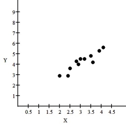 If a linear model is considered,the regression analysis is as follows: Dependent variable: Y
R-squared = 84.7%
VARIABLE COEFFICIENT
Intercept 1.2305
X .4443
What does the slope say about this relationship?
A)For every increase in X of 1,the corresponding average increase in Y is .4443
B)For every increase in X of .5,the corresponding average decrease in Y is .4443
C)For every increase in X of .5,the corresponding average increase in Y is .4443
D)For every increase in X of 1,the corresponding average increase in Y is 1.2305
E)For every increase in X of 1,the corresponding average decrease in Y is .4443
If a linear model is considered,the regression analysis is as follows: Dependent variable: YR-squared = 84.7%
VARIABLE COEFFICIENT
Intercept 1.2305
X .4443
What does the slope say about this relationship?
A)For every increase in X of 1,the corresponding average increase in Y is .4443
B)For every increase in X of .5,the corresponding average decrease in Y is .4443
C)For every increase in X of .5,the corresponding average increase in Y is .4443
D)For every increase in X of 1,the corresponding average increase in Y is 1.2305
E)For every increase in X of 1,the corresponding average decrease in Y is .4443
Question
Question
Question
Question
Question
Question
One of the important factors determining a car's fuel efficiency is its weight.This relationship is examined for 11 cars,and the association is shown in the scatterplot below. 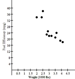 If a linear model is considered,the regression analysis is as follows: Dependent variable: MPG
R-squared = 84.7%
VARIABLE COEFFICIENT
Intercept 47.1181
Weight -7.34614
What does the slope say about this relationship?
A)Gas mileage increases an average of 7.346 mpg for each thousand pounds of weight.
B)Gas mileage decreases an average of 7.346 mpg for each thousand pounds of weight.
C)Gas mileage increases an average of 4.712 mpg for each thousand pounds of weight.
D)Gas mileage decreases an average of 4.712 mpg for each thousand pounds of weight.
E)Gas mileage decreases an average of .7346 mpg for each thousand pounds of weight.
If a linear model is considered,the regression analysis is as follows: Dependent variable: MPGR-squared = 84.7%
VARIABLE COEFFICIENT
Intercept 47.1181
Weight -7.34614
What does the slope say about this relationship?
A)Gas mileage increases an average of 7.346 mpg for each thousand pounds of weight.
B)Gas mileage decreases an average of 7.346 mpg for each thousand pounds of weight.
C)Gas mileage increases an average of 4.712 mpg for each thousand pounds of weight.
D)Gas mileage decreases an average of 4.712 mpg for each thousand pounds of weight.
E)Gas mileage decreases an average of .7346 mpg for each thousand pounds of weight.
Question
Question
Question
Question
Question
Question
Question
Question
Question
Question
Question
Question
Question
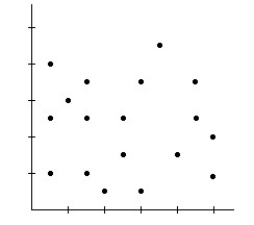
A)Model is appropriate.
B)Model may not be appropriate.The spread is changing.
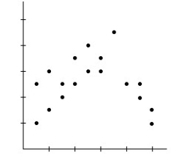
C)Model is not appropriate.The relationship is nonlinear.
Question
Question
Question
Question
Question
Question
A)Model may not be appropriate.The spread is changing.
B)Model is not appropriate.The relationship is nonlinear.
C)Model is appropriate.
Question
Question
Question
Question
A)Model is not appropriate.The relationship is nonlinear.
B)Model is appropriate.
C)Model may not be appropriate.The spread is changing.
Question
Question
Question
Question
Question
Question
A)Model may not be appropriate.The spread is changing.
B)Model is appropriate.
C)Model is not appropriate.The relationship is nonlinear.
Question
Question
Question
Question
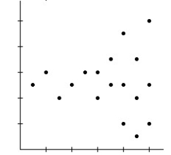
Doctors studying how the human body assimilates medication inject some patients with penicillin,and then monitor the concentration of the drug (in units/cc)in the patients' blood for seven hours.The researchers try model,using the re-expression log(Concentration).Examine the regression analysis and the residuals plot below.Explain why you think this model is appropriate. 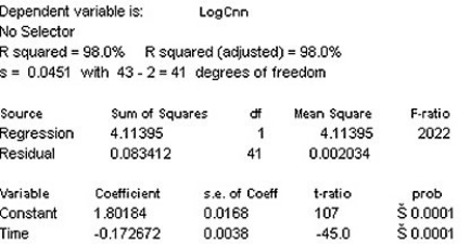
Question
Question
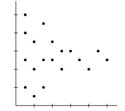
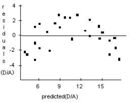
A forester would like to know how big a maple tree might be at age 50 years.She gathers data from some trees that have been cut down,and plots the diameters (in inches)of the trees against their ages (in years).First she makes a linear model.The scatterplot and residuals plot are shown.Do you think the linear model is appropriate? Explain. 
Question
Question
Question
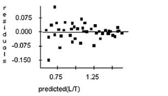
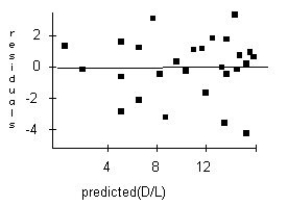
A forester would like to know how big a maple tree might be at age 50 years.She gathers data from some trees that have been cut down,and plots the diameters (in inches)of the trees against their ages (in years).She re-expresses the data,using the logarithm of age to try to predict the diameter of the tree.Here are the regression analysis and the residuals plot.Explain why you think this is an appropriate model. 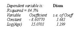
Question
One of the important factors determining a car's fuel efficiency is its weight.This relationship is examined for 11 cars,and the association is shown in the scatterplot below. 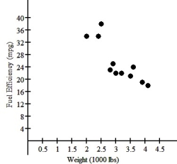 If a linear model is considered,the regression analysis is as follows: Dependent variable: MPG
R-squared = 84.7%
VARIABLE COEFFICIENT
Intercept 47.1181
Weight -7.34614
The residuals plot is: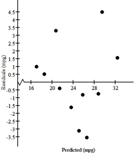 Based upon the residuals plot,do you think that this linear model is appropriate?
A)Yes,residuals show no pattern.
B)Yes,residuals show a linear pattern.
C)No,residuals show a curved pattern.
D)No,residuals show no pattern.
E)Yes,residuals show a curved pattern.
If a linear model is considered,the regression analysis is as follows: Dependent variable: MPGR-squared = 84.7%
VARIABLE COEFFICIENT
Intercept 47.1181
Weight -7.34614
The residuals plot is:
Based upon the residuals plot,do you think that this linear model is appropriate?A)Yes,residuals show no pattern.
B)Yes,residuals show a linear pattern.
C)No,residuals show a curved pattern.
D)No,residuals show no pattern.
E)Yes,residuals show a curved pattern.
Question
Question
A)Model is not appropriate.The relationship is nonlinear.
B)Model is appropriate.
C)Model may not be appropriate.The spread is changing.
Question
Question
Question
Question
Question
Question
Question
Question
A forester would like to know how big a maple tree might be at age 50 years.She gathers data from some trees that have been cut down,and plots the diameters (in inches)of the trees against their ages (in years).First she makes a linear model.The scatterplot and residuals plot are shown.If she uses this model to try to predict the diameter of a 50-year old maple tree,would you expect that estimate to be fairly accurate,too low,or too high? Explain. 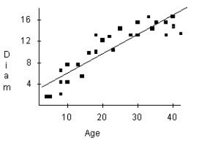

Question
Question
Doctors studying how the human body assimilates medication inject some patients with penicillin,and then monitor the concentration of the drug (in units/cc)in the patients' blood for seven hours.First they tried to fit a linear model.The regression analysis and residuals plot are shown.Is that estimate likely to be accurate,too low,or too high? Explain. 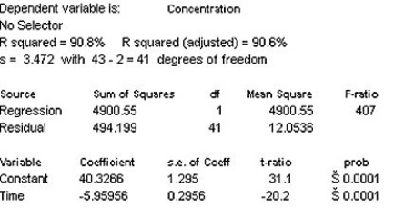
Question
A)Model may not be appropriate.The spread is changing.
B)Model is appropriate.
C)Model is not appropriate.The relationship is nonlinear.
Question
Question
Question
Question
Question
Question
Question
Question
Question
Question
Question

Unlock Deck
Sign up to unlock the cards in this deck!
Unlock Deck
Unlock Deck
1/71
Play
Full screen (f)
Deck 7: Linear Regression
1
A golf ball is dropped from 15 different heights (in cm)and the height of the bounce is recorded (in cm.)The regression analysis gives the model drop.Predict the height of the bounce if dropped from 64 cm.
A)44.9 cm
B)91.57 cm
C)44.7 cm
D)64.6 cm
E)44.8 cm
A)44.9 cm
B)91.57 cm
C)44.7 cm
D)64.6 cm
E)44.8 cm
44.7 cm
2
The relationship between two quantities X and Y is examined,and the association is shown in the scatterplot below. If a linear model is considered,the regression analysis is as follows: Dependent variable: Y
R-squared = 84.7%
VARIABLE COEFFICIENT
Intercept 1.2305
X .4443
What does the slope say about this relationship?
A)For every increase in X of 1,the corresponding average increase in Y is .4443
B)For every increase in X of .5,the corresponding average decrease in Y is .4443
C)For every increase in X of .5,the corresponding average increase in Y is .4443
D)For every increase in X of 1,the corresponding average increase in Y is 1.2305
E)For every increase in X of 1,the corresponding average decrease in Y is .4443
If a linear model is considered,the regression analysis is as follows: Dependent variable: YR-squared = 84.7%
VARIABLE COEFFICIENT
Intercept 1.2305
X .4443
What does the slope say about this relationship?
A)For every increase in X of 1,the corresponding average increase in Y is .4443
B)For every increase in X of .5,the corresponding average decrease in Y is .4443
C)For every increase in X of .5,the corresponding average increase in Y is .4443
D)For every increase in X of 1,the corresponding average increase in Y is 1.2305
E)For every increase in X of 1,the corresponding average decrease in Y is .4443
For every increase in X of 1,the corresponding average increase in Y is .4443
3
A golf ball is dropped from 15 different heights (in cm)and the height of the bounce is recorded (in cm.)The regression analysis gives the model drop.Explain what the slope of the line says about the bounce height and the drop height of the ball.
A)On average,the bounce height will be 0.69 cm less than the drop height.
B)On average,the drop height increases by 0.69 cm for every extra cm of bounce height.
C)On average,the bounce height increases by -0.3 cm for every extra cm of drop height.
D)On average,the bounce height increases by 0.69 cm for every extra cm of drop height.
E)On average,the drop height increases by -0.3 cm for every extra cm of bounce height.
On average,the bounce height increases by 0.69 cm for every extra cm of drop height.
4
The relationship between the number of games won by an NHL team and the average attendance at their home games is analyzed.A regression analysis to predict the average attendance from the number of games won gives the model wins.Predict the average attendance of a team with 58 wins.
A)11 people
B)9094 people
C)13,294 people
D)11,194 people
E)-1849 people
A)11 people
B)9094 people
C)13,294 people
D)11,194 people
E)-1849 people
Unlock Deck
Unlock for access to all 71 flashcards in this deck.
Unlock Deck
k this deck
5
A sociology student does a study to determine whether people who exercise live longer.He claims that someone who exercises 7 days a week will live 15 years longer than someone who doesn't exercise at all.
A)Predictions based on a regression line are for average values of x and y.The actual average life expectancy changes every year so an accurate prediction is impossible.
B)There is nothing wrong with the interpretation.
C)Predictions based on a regression line are for average values of y for a given x.The actual life expectancy will vary around the prediction.
D)The has to be greater than 90% to make a statement like this.
E)A linear model is inappropriate for sociology studies.
Unlock Deck
Unlock for access to all 71 flashcards in this deck.
Unlock Deck
k this deck
6
A random sample of records of electricity usage of homes gives the amount of electricity used in July and size (in square feet)of 135 homes.A regression was done to predict the amount of electricity used (in kilowatt-hours)from size.Suppose the linear model is appropriate.The model is size.Explain what the slope of the line says about the electricity usage and home size.
A)On average,the amount of electricity used increases by 1248 kilowatt-hours when the size of the house is increased by a square foot.
B)On average,the size of the house increases by 1248 feet for every kilowatt-hour used.
C)On average,the amount of electricity used is 0.6 kilowatt hours less than the size of the house.
D)On average,the amount of electricity used increases by 0.6 kilowatt-hours when the size of the house is increased by a square foot.
E)On average,the size of the house increases by 0.6 feet for every kilowatt-hour used.
Unlock Deck
Unlock for access to all 71 flashcards in this deck.
Unlock Deck
k this deck
7
A random sample of records of electricity usage of homes gives the amount of electricity used in July and size (in square feet)of 135 homes.A regression was done to predict the amount of electricity used (in kilowatt-hours)from size.Suppose the linear model is appropriate.Do you think the slope is positive or negative? Why?
A)Negative.Larger homes should use less electricity.
B)Positive.The larger the number of houses the more electricity used.
C)Negative.Smaller homes should use less electricity.
D)Positive.More square feet indicates more houses.
E)Positive.Larger homes should use more electricity.
A)Negative.Larger homes should use less electricity.
B)Positive.The larger the number of houses the more electricity used.
C)Negative.Smaller homes should use less electricity.
D)Positive.More square feet indicates more houses.
E)Positive.Larger homes should use more electricity.
Unlock Deck
Unlock for access to all 71 flashcards in this deck.
Unlock Deck
k this deck
8
One of the important factors determining a car's fuel efficiency is its weight.This relationship is examined for 11 cars,and the association is shown in the scatterplot below. If a linear model is considered,the regression analysis is as follows: Dependent variable: MPG
R-squared = 84.7%
VARIABLE COEFFICIENT
Intercept 47.1181
Weight -7.34614
What does the slope say about this relationship?
A)Gas mileage increases an average of 7.346 mpg for each thousand pounds of weight.
B)Gas mileage decreases an average of 7.346 mpg for each thousand pounds of weight.
C)Gas mileage increases an average of 4.712 mpg for each thousand pounds of weight.
D)Gas mileage decreases an average of 4.712 mpg for each thousand pounds of weight.
E)Gas mileage decreases an average of .7346 mpg for each thousand pounds of weight.
If a linear model is considered,the regression analysis is as follows: Dependent variable: MPGR-squared = 84.7%
VARIABLE COEFFICIENT
Intercept 47.1181
Weight -7.34614
What does the slope say about this relationship?
A)Gas mileage increases an average of 7.346 mpg for each thousand pounds of weight.
B)Gas mileage decreases an average of 7.346 mpg for each thousand pounds of weight.
C)Gas mileage increases an average of 4.712 mpg for each thousand pounds of weight.
D)Gas mileage decreases an average of 4.712 mpg for each thousand pounds of weight.
E)Gas mileage decreases an average of .7346 mpg for each thousand pounds of weight.
Unlock Deck
Unlock for access to all 71 flashcards in this deck.
Unlock Deck
k this deck
9
A random sample of records of electricity usage of homes in the month of July gives the amount of electricity used and size (in square feet)of 135 homes.A regression was done to predict the amount of electricity used (in kilowatt-hours)from size.Suppose the linear model is appropriate.The model is size.How much electricity would you predict would be used in a house that is 2372 square feet?
A)54 kilowatt-hours
B)2264.00 kilowatt-hours
C)1186 kilowatt-hours
D)2426 kilowatt-hours
E)3612.5 kilowatt-hours
A)54 kilowatt-hours
B)2264.00 kilowatt-hours
C)1186 kilowatt-hours
D)2426 kilowatt-hours
E)3612.5 kilowatt-hours
Unlock Deck
Unlock for access to all 71 flashcards in this deck.
Unlock Deck
k this deck
10
A random sample of records of electricity usage of homes gives the amount of electricity used in July and size (in square feet)of 135 homes.A regression to predict the amount of electricity used (in kilowatt-hours)from size was completed.What are the variables and units in this regression?
A)Amount of electricity used (in kilowatt-hours)is y and size (in square feet)is x.
B)Amount of electricity used (in kilowatt-hours)is y and number of homes is x.
C)Size (in square feet)is y and amount of electricity used (in kilowatt-hours)is x.
D)Size (in square feet)is y and number of homes is x.
E)Number of homes is y and amount of electricity used (in kilowatt-hours)is x.
Unlock Deck
Unlock for access to all 71 flashcards in this deck.
Unlock Deck
k this deck
11
The relationship between the selling price (in dollars)of used Ford Escorts and their age (in years)is analyzed.A regression analysis to predict the price from the age gives the model age.You want to sell a 17-year-old Escort.Use the model to determine an appropriate price.Explain any problems.
A)-$22,916 You won't sell a car for a negative amount.The model doesn't give meaningful prices for Escorts this old.
B)$11 The car should be worth more than this.
C)-$37,126 There are no problems with this prediction.
D)$22,916 There is no way the car is worth this much.
E)-$8706 You won't sell a car for a negative amount.The model doesn't give meaningful prices for Escorts this old.
Unlock Deck
Unlock for access to all 71 flashcards in this deck.
Unlock Deck
k this deck
12
The relationship between two quantities x and y is examined.The relationship appears to be fairly linear.A linear model is considered,and the regression analysis is as follows: Dependent variable: y
R-squared = 87.9%
VARIABLE COEFFICIENT
Intercept 37.74
X -9.97
What does the slope say about the relationship between x and y?
A)For each increase in x of 1,the corresponding average decrease in y is 9.97.
B)For each increase in x of 1,the corresponding average increase in y is 37.74.
C)For each increase in x of 1,the corresponding average decrease in y is 37.74.
D)For each increase in x of 1,the corresponding average increase in y is 9.97.
E)For each increase in x of 1,y decreases by an average of 87.9%.
Unlock Deck
Unlock for access to all 71 flashcards in this deck.
Unlock Deck
k this deck
13
A golf ball is dropped from 15 different heights (in cm)and the height of the bounce is recorded (in cm.)The regression analysis gives the model = 0.3 + 0.71 drop.Interpret the meaning of the y-intercept.
A)According to the model,a ball dropped from 0.71 cm high will bounce 0 cm.(This may not actually happen.)
B)According to the model,a ball dropped from 0.3 cm high will bounce 0 cm.(This may not actually happen.)
C)According to the model,a ball dropped from 0 cm high will bounce 0.71 cm.(This may not actually happen.)
D)According to the model,a ball dropped from 0.71 cm high will bounce 0.3 cm.(This may not actually happen.)
E)According to the model,a ball dropped from 0 cm high will bounce 0.3 cm.(This may not actually happen.)
Unlock Deck
Unlock for access to all 71 flashcards in this deck.
Unlock Deck
k this deck
14
A) = 0.6 + 14.2x
B) = 2 + 1.69x
C) = -4 + 2x
D) = 14.2 + 0.6x
E) = 20.05 + 0.15x
Unlock Deck
Unlock for access to all 71 flashcards in this deck.
Unlock Deck
k this deck
15
A)2
B)4
C)3
D)9
E)7
Unlock Deck
Unlock for access to all 71 flashcards in this deck.
Unlock Deck
k this deck
16
Consider the four points (20,20),(30,50),(40,30),and (50,60).The least squares line is Explain what "least squares" means using these data as a specific example.
A)The line = 5 + 50x minimizes the sum of the vertical distances from the points to the line.
B)The line = 5 + 50x minimizes the sum of the squared vertical distances from the points to the line.
C)The line = 5 + 50x minimizes the sum of the squared horizontal distances from the points to the line.
D)The line = 5 + 50x minimizes the square of the standard deviation.
E)The line = 5 + 50x minimizes the sum of the squared difference between the x and y values.
Unlock Deck
Unlock for access to all 71 flashcards in this deck.
Unlock Deck
k this deck
17
The relationship between the number of games won during one season by an NHL team and the average attendance at their home games is analyzed.A regression analysis to predict the average attendance from the number of games won gives the model wins.Predict the average attendance of a team with 400 wins.Explain any possible problems with this prediction.
A)13 people.There are other factors besides number of games won.
B)72,700 people.A team doesn't play that many games and their arenas probably can't hold that many people.
C)5380 people.There is no problem with this prediction.
D)76,900 people.A team doesn't play that many games and their arenas probably can't hold that many people.
E)74,800 people.It is only an estimate.
Unlock Deck
Unlock for access to all 71 flashcards in this deck.
Unlock Deck
k this deck
18
A random sample of records of electricity usage of homes gives the amount of electricity used in July and size (in square feet)of 135 homes.A regression was done to predict the amount of electricity used (in kilowatt-hours)from size.Suppose the linear model is appropriate.What units does the slope have?
A)Slope is kilowatt-hours per square foot.
B)Slope is kilowatt-hours per house.
C)Slope is square feet per kilowatt-hour.
D)Slope is square feet per house.
E)Slope is houses per kilowatt-hour.
A)Slope is kilowatt-hours per square foot.
B)Slope is kilowatt-hours per house.
C)Slope is square feet per kilowatt-hour.
D)Slope is square feet per house.
E)Slope is houses per kilowatt-hour.
Unlock Deck
Unlock for access to all 71 flashcards in this deck.
Unlock Deck
k this deck
19
The relationship between the selling price (in dollars)of used Ford Escorts and their age (in years)is analyzed.A regression analysis to predict the price from the age gives the model age.Predict the price of an Escort that is 8 years old.
A)$11,776
B)$10
C)$26,234
D)$12,994
E)$2682
A)$11,776
B)$10
C)$26,234
D)$12,994
E)$2682
Unlock Deck
Unlock for access to all 71 flashcards in this deck.
Unlock Deck
k this deck
20
A random sample of 150 yachts sold in the Canada last year was taken.A regression analysis to predict the price (in thousands of dollars)from length (in metres)was completed.A linear model is appropriate.What are the units of the slope?
A)Slope is yachts per dollar.
B)Slope is metres per dollar.
C)Slope is dollars per metre.
D)Slope is metres per thousand dollars.
E)Slope is thousands of dollars per metre.
A)Slope is yachts per dollar.
B)Slope is metres per dollar.
C)Slope is dollars per metre.
D)Slope is metres per thousand dollars.
E)Slope is thousands of dollars per metre.
Unlock Deck
Unlock for access to all 71 flashcards in this deck.
Unlock Deck
k this deck
21
A)Model is appropriate.
B)Model may not be appropriate.The spread is changing.
C)Model is not appropriate.The relationship is nonlinear.
Unlock Deck
Unlock for access to all 71 flashcards in this deck.
Unlock Deck
k this deck
22
A golf ball was dropped from 8 different heights.The drop height and the bounce height were recorded.
A) = 73 - .765 drop
B) = -0.335 + 1.305 drop
C) = 0.321 + .765 drop
D) = 95 - 9.1 drop
E) = 0.215 + .866 drop
A) = 73 - .765 drop
B) = -0.335 + 1.305 drop
C) = 0.321 + .765 drop
D) = 95 - 9.1 drop
E) = 0.215 + .866 drop
Unlock Deck
Unlock for access to all 71 flashcards in this deck.
Unlock Deck
k this deck
23
A) = 79.40 - 24.00x
B) = 40.00 + 2.47x
C) = -24.00 + 79.40x
D) = -112.60 + 40.00x
E) = 7.45 - 0.01x
Unlock Deck
Unlock for access to all 71 flashcards in this deck.
Unlock Deck
k this deck
24
The relationship between the number of games won by an NHL team (x)and the average attendance at their home games (y)is analyzed.The mean number of games won was 70 with a standard deviation of 16.The mean attendance was 6993 with a standard deviation of 1400.The correlation between the games won and attendance was 0.47.
A) = 4114 + 41.125 wins
B) = 2360 + 66.1 wins
C) = 6990 + 0.00537 wins
D) = 868 + 87.5 wins
E) = -2890 + 141 wins
A) = 4114 + 41.125 wins
B) = 2360 + 66.1 wins
C) = 6990 + 0.00537 wins
D) = 868 + 87.5 wins
E) = -2890 + 141 wins
Unlock Deck
Unlock for access to all 71 flashcards in this deck.
Unlock Deck
k this deck
25
Two different tests are designed to measure employee productivity and dexterity.Several employees are randomly selected and tested with these results. Dexterity
Productivity
A) = 2.36 + 2.03 Dexterity
B) = 6.08 + 1.56 Dexterity
C) = 75.3 - 0.329 Dexterity
D) = 10.7 + 1.53 Dexterity
E) = 5.05 + 1.91 Dexterity
Productivity
A) = 2.36 + 2.03 Dexterity
B) = 6.08 + 1.56 Dexterity
C) = 75.3 - 0.329 Dexterity
D) = 10.7 + 1.53 Dexterity
E) = 5.05 + 1.91 Dexterity
Unlock Deck
Unlock for access to all 71 flashcards in this deck.
Unlock Deck
k this deck
26
A) = 12.25; = 0.90
B) = -46; = 11.50
C) = 49; = -14.25
D) = 11; = 1.80
E) = 2.75; = 0.45
Unlock Deck
Unlock for access to all 71 flashcards in this deck.
Unlock Deck
k this deck
27
A)Model may not be appropriate.The spread is changing.
B)Model is not appropriate.The relationship is nonlinear.
C)Model is appropriate.
Unlock Deck
Unlock for access to all 71 flashcards in this deck.
Unlock Deck
k this deck
28
Ten Ford Escort classified ads were selected.The age and prices of several used Ford Escorts are given in the table.
A) = 11291 - 1578 age
B) = 7200 - 692 age
C) = 7.05 -0.000616 age
D) = -1580 + 11300 age
E) = 10000 - 1600 age
A) = 11291 - 1578 age
B) = 7200 - 692 age
C) = 7.05 -0.000616 age
D) = -1580 + 11300 age
E) = 10000 - 1600 age
Unlock Deck
Unlock for access to all 71 flashcards in this deck.
Unlock Deck
k this deck
29
If the linear correlation between typical daily temperature and coat sales is -0.737 and today the temperature is 2 standard deviations above the mean,what would you predict coat sales to be with respect to its mean?
A)2.000 standard deviations below the mean sales
B)1.474 standard deviations above the mean sales
C)2.000 standard deviations above the mean sales
D)1.474 standard deviations below the mean sales
E)0.737 standard deviations below the mean height
A)2.000 standard deviations below the mean sales
B)1.474 standard deviations above the mean sales
C)2.000 standard deviations above the mean sales
D)1.474 standard deviations below the mean sales
E)0.737 standard deviations below the mean height
Unlock Deck
Unlock for access to all 71 flashcards in this deck.
Unlock Deck
k this deck
30
If the linear correlation between shoe size and height is 0.758 and Dave is 2 standard deviations above the mean in shoe size,what would you predict is Dave's height with respect to the mean height?
A)2.000 standard deviations above the mean height
B)1.516 standard deviations above the mean height
C)0.575 standard deviations above the mean height
D)0.758 standard deviations above the mean height
E)1.149 standard deviations above the mean height
A)2.000 standard deviations above the mean height
B)1.516 standard deviations above the mean height
C)0.575 standard deviations above the mean height
D)0.758 standard deviations above the mean height
E)1.149 standard deviations above the mean height
Unlock Deck
Unlock for access to all 71 flashcards in this deck.
Unlock Deck
k this deck
31
A)Model is not appropriate.The relationship is nonlinear.
B)Model is appropriate.
C)Model may not be appropriate.The spread is changing.
Unlock Deck
Unlock for access to all 71 flashcards in this deck.
Unlock Deck
k this deck
32
Ten Jeep Cherokee classified ads were selected.The age and prices of several used Ford Escorts are given in the table.
A) = 7.05 -0.000319 age
B) = -3110 + 22000 age
C) = 21979 - 3108 age
D) = 17200 - 891 age
E) = 19000 - 3000 age
A) = 7.05 -0.000319 age
B) = -3110 + 22000 age
C) = 21979 - 3108 age
D) = 17200 - 891 age
E) = 19000 - 3000 age
Unlock Deck
Unlock for access to all 71 flashcards in this deck.
Unlock Deck
k this deck
33
Ten students in a graduate program at Carleton University were randomly selected.Their grade point averages (GPAs)when they entered the program were between 11.5 and 12.0.The following data were obtained regarding their GPAs on entering the program versus their current GPAs.
A) = 10.51 + 0.329E
B) =12.23 + 0.746E
C) = 11.42 + 0.0312E
D) = 13.81 + 0.497E
E) = 12.91 + 0.0212E
A) = 10.51 + 0.329E
B) =12.23 + 0.746E
C) = 11.42 + 0.0312E
D) = 13.81 + 0.497E
E) = 12.91 + 0.0212E
Unlock Deck
Unlock for access to all 71 flashcards in this deck.
Unlock Deck
k this deck
34
Managers rate employees according to job performance and attitude.The results for several randomly selected employees are given below. Attitude
Performance
A) = 100.3 - 0.453 Attitude
B) = 92.3 - 0.669 Attitude
C) = 2.81 + 1.35 Attitude
D) = -47.3 + 2.02 Attitude
E)11. = 11.7 + 1.02 Attitude
Performance
A) = 100.3 - 0.453 Attitude
B) = 92.3 - 0.669 Attitude
C) = 2.81 + 1.35 Attitude
D) = -47.3 + 2.02 Attitude
E)11. = 11.7 + 1.02 Attitude
Unlock Deck
Unlock for access to all 71 flashcards in this deck.
Unlock Deck
k this deck
35
Ten students in a tutor program at Carleton University were randomly selected.Their grade point averages (GPAs)when they entered the program were less than 9.5.The following data were obtained regarding their GPAs on entering the program versus their current GPAs.
A) = 0.711 + 0.346E
B) = 0.873 + 0.627E
C) = 2.51 + 0.529E
D) = 1.54 + 0.8566E
E) = 0.0065 + 0.879E
A) = 0.711 + 0.346E
B) = 0.873 + 0.627E
C) = 2.51 + 0.529E
D) = 1.54 + 0.8566E
E) = 0.0065 + 0.879E
Unlock Deck
Unlock for access to all 71 flashcards in this deck.
Unlock Deck
k this deck
36
A) = 220; = 12.50
B) = 190; = 0.32
C) = 210; = 6
D) = 180; = 12.50
E) = 20; = 2.50
Unlock Deck
Unlock for access to all 71 flashcards in this deck.
Unlock Deck
k this deck
37
A)Model may not be appropriate.The spread is changing.
B)Model is appropriate.
C)Model is not appropriate.The relationship is nonlinear.
Unlock Deck
Unlock for access to all 71 flashcards in this deck.
Unlock Deck
k this deck
38
The relationship between the cost of a taxi ride (y)and the length of the ride (x)is analyzed.The mean length was 4.6 km with a standard deviation of 1.1.The mean cost was $8.70 with a standard deviation of 2.0.The correlation between the cost and the length was 0.81.
A) = 0.336 + 1.82 length
B) = 1.93 + 1.47 length
C) = -113 + 26.5 length
D) = 6.65 + 0.446 length
E) = -458 + 101 length
A) = 0.336 + 1.82 length
B) = 1.93 + 1.47 length
C) = -113 + 26.5 length
D) = 6.65 + 0.446 length
E) = -458 + 101 length
Unlock Deck
Unlock for access to all 71 flashcards in this deck.
Unlock Deck
k this deck
39
The relationship between the price of yachts (y)and their length (x)is analyzed.The mean length was 41 metres with a standard deviation of 11.The mean price was $84,000 with a standard deviation of 14,000.The correlation between the price and the length was 0.41.
A) = 31,800 + 1270 length
B) = 70,800 + 0.000322 length
C) = -962,000 + 547 length
D) = -4,040,000 + 622 length
E) = 62,605+ 522 length
A) = 31,800 + 1270 length
B) = 70,800 + 0.000322 length
C) = -962,000 + 547 length
D) = -4,040,000 + 622 length
E) = 62,605+ 522 length
Unlock Deck
Unlock for access to all 71 flashcards in this deck.
Unlock Deck
k this deck
40
A) = 60; r = 0.60
B) = 180; r = -0.60
C) = -117; r = 0.50
D) = -48; r = 0.03
E) = -300; r = 0.50
Unlock Deck
Unlock for access to all 71 flashcards in this deck.
Unlock Deck
k this deck
41
Doctors studying how the human body assimilates medication inject some patients with penicillin,and then monitor the concentration of the drug (in units/cc)in the patients' blood for seven hours.The researchers try model,using the re-expression log(Concentration).Examine the regression analysis and the residuals plot below.Explain why you think this model is appropriate.
Unlock Deck
Unlock for access to all 71 flashcards in this deck.
Unlock Deck
k this deck
42
The relationship between the number of games won by an NHL team and the average attendance at their home games is analyzed.A regression analysis to predict the average attendance from the number of games won gives the model wins.One team averaged 4240 fans at each game.They won 57 times.Calculate the residual and explain what it means.
A)17,272 people.The team averaged 17,272 less fans than would be predicted for a team with 57 wins.
B)2792 people.The team averaged 2792 more fans than would be predicted for a team with 57 wins.
C)-2792 people.The team averaged 2792 less fans than would be predicted for a team with 57 wins.
D)4223 people.On average the team will have 4223 extra people.
E)7032 people.The team was expected to average 7032 people for each game.
Unlock Deck
Unlock for access to all 71 flashcards in this deck.
Unlock Deck
k this deck
43
A forester would like to know how big a maple tree might be at age 50 years.She gathers data from some trees that have been cut down,and plots the diameters (in inches)of the trees against their ages (in years).First she makes a linear model.The scatterplot and residuals plot are shown.Do you think the linear model is appropriate? Explain.
Unlock Deck
Unlock for access to all 71 flashcards in this deck.
Unlock Deck
k this deck
44
The relationship between the number of games won by an NHL team and the average attendance at their home games is analyzed.A regression to predict the average attendance from the number of games won has an = 30.4%.The residuals plot indicated that a linear model is appropriate.Write a sentence summarizing what says about this regression.
A)Differences in average attendance explain 30.4% of the variation in the number of games won.
B)In 30.4% of games won the attendance was at least as large as the average attendance.
C)The number of games won explains 69.6% of the variation in average attendance.
D)The number of games won explains 30.4% of the variation in average attendance.
E)Differences in average attendance explain 69.6% of the variation in the number of games won.
Unlock Deck
Unlock for access to all 71 flashcards in this deck.
Unlock Deck
k this deck
45
A random sample of records of electricity usage of homes in the month of July gives the amount of electricity used and size (in square feet)of 135 homes.A regression was done to predict the amount of electricity used (in kilowatt-hours)from size.The residuals plot indicated that a linear model is appropriate.The model is size.The people in a house that is 2347 square feet used 500 kilowatt-hours less than expected.How much did they use?
A)1491.1 kilowatt-hours
B)3134.3 kilowatt-hours
C)-82.9 kilowatt-hours
D)3533.33 kilowatt-hours
E)1204.1 kilowatt-hours
A)1491.1 kilowatt-hours
B)3134.3 kilowatt-hours
C)-82.9 kilowatt-hours
D)3533.33 kilowatt-hours
E)1204.1 kilowatt-hours
Unlock Deck
Unlock for access to all 71 flashcards in this deck.
Unlock Deck
k this deck
46
A forester would like to know how big a maple tree might be at age 50 years.She gathers data from some trees that have been cut down,and plots the diameters (in inches)of the trees against their ages (in years).She re-expresses the data,using the logarithm of age to try to predict the diameter of the tree.Here are the regression analysis and the residuals plot.Explain why you think this is an appropriate model.
Unlock Deck
Unlock for access to all 71 flashcards in this deck.
Unlock Deck
k this deck
47
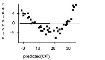
One of the important factors determining a car's fuel efficiency is its weight.This relationship is examined for 11 cars,and the association is shown in the scatterplot below. If a linear model is considered,the regression analysis is as follows: Dependent variable: MPG
R-squared = 84.7%
VARIABLE COEFFICIENT
Intercept 47.1181
Weight -7.34614
The residuals plot is: Based upon the residuals plot,do you think that this linear model is appropriate?
A)Yes,residuals show no pattern.
B)Yes,residuals show a linear pattern.
C)No,residuals show a curved pattern.
D)No,residuals show no pattern.
E)Yes,residuals show a curved pattern.
If a linear model is considered,the regression analysis is as follows: Dependent variable: MPGR-squared = 84.7%
VARIABLE COEFFICIENT
Intercept 47.1181
Weight -7.34614
The residuals plot is:
Based upon the residuals plot,do you think that this linear model is appropriate?A)Yes,residuals show no pattern.
B)Yes,residuals show a linear pattern.
C)No,residuals show a curved pattern.
D)No,residuals show no pattern.
E)Yes,residuals show a curved pattern.
Unlock Deck
Unlock for access to all 71 flashcards in this deck.
Unlock Deck
k this deck
48
A golf ball is dropped from 15 different heights (in cm)and the height of the bounce is recorded (in cm).The regression analysis gives the model drop.A golf ball dropped from 61 cm bounced a height whose residual is -1.8 cm.What is the bounce height?
A)1.8 cm
B)59.45 cm
C)59.2 cm
D)47.35 cm
E)43.75 cm
A)1.8 cm
B)59.45 cm
C)59.2 cm
D)47.35 cm
E)43.75 cm
Unlock Deck
Unlock for access to all 71 flashcards in this deck.
Unlock Deck
k this deck
49
A)Model is not appropriate.The relationship is nonlinear.
B)Model is appropriate.
C)Model may not be appropriate.The spread is changing.
Unlock Deck
Unlock for access to all 71 flashcards in this deck.
Unlock Deck
k this deck
50
A golf ball is dropped from 15 different heights (in cm)and the height of the bounce is recorded (in cm).The regression analysis gives the model drop.A golf ball company is trying to show that its new ball will increase your driving distance.If the new ball is dropped from several heights would the company rather see positive or negative residuals.Explain.
A)Negative.The ball isn't bouncing as high as expected so you would more likely be able to hit it longer.
B)Positive.This would mean the ball is bouncing more than expected and you would more likely be able to hit it longer.
C)Positive.This would mean the ball is being dropped from higher distances so you would more likely be able to hit it longer.
D)Neither.The ball should bounce the same as expected otherwise it wasn't manufactured properly.
E)Negative.This would mean the ball is bouncing more than expected and you would more likely be able to hit it longer.
Unlock Deck
Unlock for access to all 71 flashcards in this deck.
Unlock Deck
k this deck
51
The relationship between the number of games won by an NHL team and the average attendance at their home games is analyzed.A regression analysis to predict the average attendance from the number of games won gives the model wins.One team averaged 14,865 fans at each game and won 49 times.Calculate the residual for this team and explain what it means.
A)14,853 people.On average the team will have 14,853 extra people.
B)-6440 people.The team averaged 6440 less fans than would be predicted for a team with 49 wins.
C)28,490 people.The team averaged 28,490 more fans than would be predicted for a team with 49 wins.
D)6440 people.The team averaged 6440 more fans than would be predicted for a team with 49 wins.
E)8425 people.The team was expected to average 8425 people for each game.
Unlock Deck
Unlock for access to all 71 flashcards in this deck.
Unlock Deck
k this deck
52
Using advertised prices for used Ford Escorts a linear model for the relationship between a car's age and its price is found.The regression has an = 87.7%.Write a sentence summarizing what says about this regression.
A)The age of the car explains 87.7% of the variation in price.
B)The price of the car explains 87.7% of the variation in age.
C)The age of the car explains 12.3% of the variation in price.
D)The age of the car explains 9.36% of the variation in price.
E)The price of the car explains 12.3% of the variation in age.
Unlock Deck
Unlock for access to all 71 flashcards in this deck.
Unlock Deck
k this deck
53
The relationship between the number of games won by an NHL team and the average attendance at their home games is analyzed.A regression to predict the average attendance from the number of games won has an = 31.4%.The residuals plot indicated that a linear model is appropriate.What is the correlation between the average attendance and the number of games won.
A)0.099
B)0.560
C)0.314
D)0.686
E)0.828
A)0.099
B)0.560
C)0.314
D)0.686
E)0.828
Unlock Deck
Unlock for access to all 71 flashcards in this deck.
Unlock Deck
k this deck
54
A random sample of records of electricity usage of homes in the month of July gives the amount of electricity used and size (in square feet)of 135 homes.A regression was done to predict the amount of electricity used (in kilowatt-hours)from size.The residuals plot indicated that a linear model is appropriate.The model is size.What would a negative residual mean for people living in a house that is 2495 square feet?
A)They are using more electricity than expected.
B)Their house is bigger than expected.
C)Their house is smaller than expected.
D)They are using the least amount of electricity of all of the houses sampled.
E)They are using less electricity than expected.
A)They are using more electricity than expected.
B)Their house is bigger than expected.
C)Their house is smaller than expected.
D)They are using the least amount of electricity of all of the houses sampled.
E)They are using less electricity than expected.
Unlock Deck
Unlock for access to all 71 flashcards in this deck.
Unlock Deck
k this deck
55
A golf ball is dropped from 15 different heights (in cm)and the height of the bounce is recorded (in cm).The regression analysis gives the model drop.A golf ball dropped from 61 cm bounced 46.44 cm.What is the residual for this bounce height?
A)-1 cm
B)0.74 cm
C)46.14 cm
D)1 cm
E)2 cm
A)-1 cm
B)0.74 cm
C)46.14 cm
D)1 cm
E)2 cm
Unlock Deck
Unlock for access to all 71 flashcards in this deck.
Unlock Deck
k this deck
56
A random sample of records of electricity usage of homes gives the amount of electricity used and size (in square feet)of 135 homes.A regression to predict the amount of electricity used (in kilowatt-hours)from size has an R-squared of 71.3%.The residuals plot indicated that a linear model is appropriate.Write a sentence summarizing what says about this regression.
A)Size differences explain 28.7% of the variation in electricity usage.
B)Differences in electricity usage explain 71.3% of the variation in the size of house.
C)Size differences explain 71.3% of the variation in the number of homes.
D)Size differences explain 71.3% of the variation in electricity usage.
E)Differences in electricity usage explain 28.7% of the variation in the number of house.
Unlock Deck
Unlock for access to all 71 flashcards in this deck.
Unlock Deck
k this deck
57
A forester would like to know how big a maple tree might be at age 50 years.She gathers data from some trees that have been cut down,and plots the diameters (in inches)of the trees against their ages (in years).First she makes a linear model.The scatterplot and residuals plot are shown.If she uses this model to try to predict the diameter of a 50-year old maple tree,would you expect that estimate to be fairly accurate,too low,or too high? Explain.
Unlock Deck
Unlock for access to all 71 flashcards in this deck.
Unlock Deck
k this deck
58
A golf ball is dropped from 15 different heights (in cm)and the height of the bounce is recorded (in cm.)The regression analysis gives the model drop.A golf ball dropped from 64 cm bounced 1 cm less than expected.How high did it bounce?
A)86.94 cm
B)45.08 cm
C)47.48 cm
D)66.12 cm
E)45.48 cm
A)86.94 cm
B)45.08 cm
C)47.48 cm
D)66.12 cm
E)45.48 cm
Unlock Deck
Unlock for access to all 71 flashcards in this deck.
Unlock Deck
k this deck
59
Doctors studying how the human body assimilates medication inject some patients with penicillin,and then monitor the concentration of the drug (in units/cc)in the patients' blood for seven hours.First they tried to fit a linear model.The regression analysis and residuals plot are shown.Is that estimate likely to be accurate,too low,or too high? Explain.
Unlock Deck
Unlock for access to all 71 flashcards in this deck.
Unlock Deck
k this deck
60
A)Model may not be appropriate.The spread is changing.
B)Model is appropriate.
C)Model is not appropriate.The relationship is nonlinear.
Unlock Deck
Unlock for access to all 71 flashcards in this deck.
Unlock Deck
k this deck
61
When checking the "Does the Plot Thicken?" condition,which is the best graph to look at?
A)Residual plot
B)Histogram
C)Boxplot
D)Scatterplot
E)Pie Chart
A)Residual plot
B)Histogram
C)Boxplot
D)Scatterplot
E)Pie Chart
Unlock Deck
Unlock for access to all 71 flashcards in this deck.
Unlock Deck
k this deck
62
A biology student does a study to investigate the association between the amount of sunlight and the number of roses on a rosebush in one summer.(The value is 58%)He claims that the amount of sunlight determines 58% of the number of roses on a rosebush in one summer.
A)The has to be greater than 90% to make a statement like this.
B)The amount of sunlight accounts for 58% of the variation in the number of roses.It does not determine the number of roses.
C)The amount of sunlight will increase the number of roses 58% of the time.
D)The amount of variation in sunlight changes 58% of the time.This tells us nothing about the number of roses.
E)There is nothing wrong with the interpretation.
Unlock Deck
Unlock for access to all 71 flashcards in this deck.
Unlock Deck
k this deck
63
When checking the "Straight Enough" condition,which is the best graph to look at?
A)Residual plot.
B)Histogram
C)Boxplot
D)Scatterplot
E)Pie Chart
A)Residual plot.
B)Histogram
C)Boxplot
D)Scatterplot
E)Pie Chart
Unlock Deck
Unlock for access to all 71 flashcards in this deck.
Unlock Deck
k this deck
64
List all the regression assumptions and conditions described in Chapter 7 of your textbook.
Unlock Deck
Unlock for access to all 71 flashcards in this deck.
Unlock Deck
k this deck
65
The relationship between the number of games won by an NHL team and the average attendance at their home games is analyzed.A regression to predict the average attendance from the number of games won has an Interpret this statistic.
A)Negative,fairly strong linear relationship.62.41% of the variation in average attendance is explained by the number of games won.
B)Negative,weak linear relationship.4.41% of the variation in average attendance is explained by the number of games won.
C)Positive,weak linear relationship.4.41% of the variation in average attendance is explained by the number of games won.
D)Positive,fairly strong linear relationship.79% of the variation in average attendance is explained by the number of games won.
E)Positive,fairly strong linear relationship.62.41% of the variation in average attendance is explained by the number of games won.
Unlock Deck
Unlock for access to all 71 flashcards in this deck.
Unlock Deck
k this deck
66
A random sample of 150 yachts sold in Canada last year was taken.A regression to predict the price (in thousands of dollars)from length (in metres)has an What is correlation between length and price?
A)0.428
B)0.033
C)0.667
D)0.904
E)0.183
A)0.428
B)0.033
C)0.667
D)0.904
E)0.183
Unlock Deck
Unlock for access to all 71 flashcards in this deck.
Unlock Deck
k this deck
67
Using advertised prices for used Ford Escorts a linear model for the relationship between a car's age and its price is found.The regression has an = 85.8%.Why doesn't the model explain 100% of the variation in the price of an Escort?
A)The model was calculated incorrectly.It should explain all the variation in price.
B)The model is only right 85.8% of the time.
C)14.2% of the time the buyer is getting ripped off by an unscrupulous seller.
D)The prices of all used Ford Escorts were not used.
E)There are other factors besides age that affect the price.These include things such as mileage,options,and condition of the car.
Unlock Deck
Unlock for access to all 71 flashcards in this deck.
Unlock Deck
k this deck
68
A random sample of 150 yachts sold in Canada last year was taken.A regression to predict the price (in thousands of dollars)from length (in feet)has an = 19.00%.What would you predict about the price of the yacht whose length was one standard deviation above the mean?
A)The price should be 1 SD above the mean in price.
B)The price should be 0.436 SDs above the mean in price.
C)The price should be 1 SD below the mean in price.
D)The price should be 0.900 SDs above the mean in price.
E)The price should be 0.872 SDs above the mean in price.
A)The price should be 1 SD above the mean in price.
B)The price should be 0.436 SDs above the mean in price.
C)The price should be 1 SD below the mean in price.
D)The price should be 0.900 SDs above the mean in price.
E)The price should be 0.872 SDs above the mean in price.
Unlock Deck
Unlock for access to all 71 flashcards in this deck.
Unlock Deck
k this deck
69
Using advertised prices for used Ford Escorts a linear model for the relationship between a car's age and its price is found.The regression has an = 88.2%.Describe the relationship
A)Positive,strong linear relationship.As the age increases the price goes up.
B)Negative,weak linear relationship.As the age decreases the price goes down.
C)Positive,weak linear relationship.As the age increases the price goes down.
D)Negative,strong linear relationship.As the age increases the price goes down.
E)Negative,strong linear relationship.As the age increases the price stays the same.
Unlock Deck
Unlock for access to all 71 flashcards in this deck.
Unlock Deck
k this deck
70
A random sample of 150 yachts sold in Canada last year was taken.A regression to predict the price (in thousands of dollars)from length (in metres)has an What would you predict about the price of the yacht whose length was two standard deviations below the mean?
A)The price should be 0.780 SDs below the mean in price.
B)The price should be 0.390 SDs below the mean in price.
C)The price should be 1 SD below the mean in price.
D)The price should be 1.842 SDs below the mean in price.
E)The price should be 1 SD above the mean in price.
A)The price should be 0.780 SDs below the mean in price.
B)The price should be 0.390 SDs below the mean in price.
C)The price should be 1 SD below the mean in price.
D)The price should be 1.842 SDs below the mean in price.
E)The price should be 1 SD above the mean in price.
Unlock Deck
Unlock for access to all 71 flashcards in this deck.
Unlock Deck
k this deck
71
A psychologist does an experiment to determine whether an outgoing person can be identified by his or her handwriting.She claims that the of 89% shows that this linear model is appropriate.
A) does not tell whether the model is appropriate,but measures the strength of the linear relationship.High could also be due to an outlier.
B)This means that 89% of the dependent values will fall within one standard deviation of the mean and tells nothing about the appropriateness of the model.
C)An this high means there is a very weak linear association and the model is probably inappropriate.
D) does not tell whether the model is appropriate,but gives the percentage of data points that are close to the model.You can sometimes have a high with a nonlinear relationship.
E)There is nothing wrong with the interpretation.
Unlock Deck
Unlock for access to all 71 flashcards in this deck.
Unlock Deck
k this deck
Unlock Deck
Unlock for access to all 71 flashcards in this deck.


