Intermediate Microeconomics and Its Application 12th Edition by Walter Nicholson,Christopher Snyder

Exercise 18

Price Volatility
To an economist, price changes can almost always be explained by looking at supply and demand factors in a market. If you can assume that demand for a product is relatively stable, the effects of shifts in supply conditions can also tell us quite a bit about the price elasticity of demand. This possibility is illustrated in Figure 1 for two different kinds of products. For product X, demand is relatively inelastic (D Y ), whereas for product Y, demand is quite elastic (D X ) Þ. Consider now the effects of a very volatile supply situation in which the supply curve shifts back and forth among several possible positions. As Figure 1 shows, these shifts in supply will have very different consequences for changing prices depending on the nature of the demand curve. For good X, prices change dramatically when supply shifts. However, because demand is inelastic, the quantities bought are relatively stable. For good Y, this situation is reversed. In this case prices are relatively stable, whereas quantities change by a lot. Hence, evidence on prices in response to supply shifts can tell us quite a bit about the price elasticity of demand.
Farm Prices
Supply conditions for most agricultural products are highly volatile, primarily because weather conditions in growing areas can affect crop yields dramatically. Because the demand for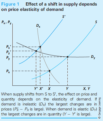
products such as corn or wheat is relatively inelastic, this can lead to highly variable prices for farm products. For example, between 2005 and 2013 an index of crop prices was as low as 110 and as high as 250, even though prices for most other products were quite stable during the period.
This inelasticity of the demand curve for farm crops leads to what is called "The Paradox of Agriculture." During periods of bad weather, crop prices rise dramatically and total spending on crops actually increases (see Table 3.2). This causes total farm income to rise-so bad weather ends up being good for many farmers. On the other hand, good weather leads to bumper crops, a large fall in crop prices, and a decline in overall farm income. Hence, TV reporters who focus on the impact of localized droughts on farm output in one area (where the farmers really are harmed) largely miss the important benefit that this confers on other farmers who have been less affected by drought conditions.
Temporary Sales
When markets are relatively competitive, the demand curve facing any one seller will be quite elastic. Consider, for example, the situation of the McDonald's restaurant chain. The chain faces many competitors, who both produce similar hamburgers (Burger King) and other closely substitutable fast foods (Kentucky Fried Chicken). When McDonald's initiates a special sales campaign (as it did in 2012 with its "dollar meals"), it can gain a large quantity of extra sales with only a small price drop. A similar situation occurs when a particular service station offers a small price reduction in gasoline prices-everyone flocks to the gas station with the lowest posted price. Of course, such effects can only last until competitors respond to these temporary sales prices. Analyzing that possibility in detail must await our modeling of market equilibrium in later chapters. But it seems clear that with such elastic demand curves, prices for fast food will be relatively stable.
Why is it important that the demand curves in Figure 1 stay in a fixed position? If demand were to shift when supply shifts, could we conclude anything about the elasticity of demand? Can you think of situations where a shift in supply is usually also accompanied by a shift in demand?