Microeconomics 2nd Edition by Douglas Bernheim

Exercise 1

Repeat Worked-Out Problem 21.1, but assume that the supply function of low-ability workers is Q L s = 0.15( W 2,000).
Worked-Out Problem 21.1

Figure 21.1 Demand and Supply for Software Programmers. The figure shows the demand and supply curves for high- and low-ability workers when ability is perfectly observable. In the competitive equilibrium, employers hire 400 low-ability workers at a wage of $6,000 per month, and 500 high-ability workers at a wage of $12,000 per month.

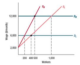
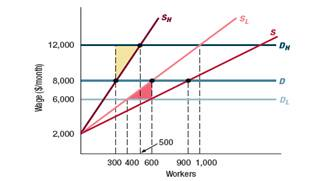
Figure 21.2 Demand and Supply for Software Programmers When Ability Is Not Observable by Employers. The figure shows the market equilibrium when employers cannot observe workers' abilities. At each wage above $2,000 per month, two-thirds of the available workers have low ability. As a result, an employer is willing to pay workers $8,000 per month, leading to the demand curve labeled D. The aggregate labor supply curve is S, the horizontal sum of the supply curves for high-ability and low-ability workers, S H and S L respectively. In the equilibrium, employers hire 900 workers at a wage of $8,000 per month. Three hundred of those workers have high ability and 600 have low ability. The deadweight loss from asymmetric information is the sum of the yellow-shaded triangle (the loss from hiring too few high-ability workers) and the red-shaded triangle (the loss from hiring too many low-ability workers).