Understanding Basic Statistics 6th Edition by Charles Henry Brase,Corrinne Pellillo Brase

Exercise 21

Draw a scatter diagram displaying the data.
(b) Verify the given sums x , y , x 2 , y 2 , and xy , and the value of the sample correlation coefficient r.
(c) Find
, a , and b. Then find the equation of the least-squares line = a + bx.
(d) Graph the least-squares line on your scatter diagram. Be sure to use the point(
) as one of the points on the line.
(e) Interpretation Find the value of the coefficient of determination r 2. What percentage of the variation in y can be explained by the corresponding variation in x and the least-squares line What percentage is unexplained Answers may vary slightly due to rounding.
Income: Medical Care Let x be per capita income in thousands of dollars. Let y be the number of medical doctors per 10,000 residents. Six small cities in Oregon gave the following information about x and y. (based on information from life in america's small cities by G.S. Thomas. Prometheus Books).

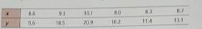
Complete parts (a) through (e), given x = 53, y = 83.7, x ² = 471,04, y ² = 1276.83, xy = 755.89, and r 0.943.
(f) Suppose a small city in Oregon has a capita income of 10 thousand dollars. What is the predicted number of M.D. s per 10,000 residents