
Understanding Basic Statistics 6th Edition by Charles Henry Brase,Corrinne Pellillo Brase
Edition 6ISBN: 978-1111827021Understanding Basic Statistics 6th Edition by Charles Henry Brase,Corrinne Pellillo Brase
Edition 6ISBN: 978-1111827021 Exercise 36
Expand Your Knowledge: Plus Four Confidence Interval for a Single Proportion One of the technical difficulties that arises in the computation of confidence intervals for a single proportion is that the exact formula for the maximal margin of error requires knowledge of the population proportionof success p. Since p is usually not known, we use the sample estimate
 = r/n in place of p. As discussed in the article "How Much Confidence Should You Have in Binomial Confidence Intervals" appearing in issue no. 45 of the magazine STATS (a publication of the American Statistical Association), use of
 as an estimate for p means that the actual confidence level for the intervals may in fact be smaller than the specified level c. This problem arises even when n is large, especially if p is not near 1/2.
A simple adjustment to the formula for the confidence intervals is the plus four estimate, first suggested by Edwin Bidwell Wilson in 1927. It is also called the Agresti-Coull confidence interval. This adjustment works best for 95% confidence intervals.
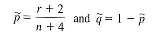
The plus four adjustment has us add two successes and two failures to the sample data. This means that r , the number of successes, is increased by 2, and n, the sample size is increased by 4. We use the symbol
 , read " P tilde, " for the resulting sample estimate of p. So,
 = (r + 2)/( n + 4)
PROCEDURE
HOW TO COMPUTE A PLUS FOUR CONFIDENCE INTERVAL FOR p
Requirements
Consider a binomial experiment with n trials, where p represents the population probability of success and q = 1 - p represents the population probability of failure. Let r be a random variable that represents the number of successes out of the n binomial trials.
The plus four point estimates for p and q are
The number of trials n should be at least 10.
Approximate confidence interval for p
 - E p
- E p
 + E
+ E
Where
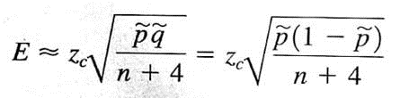
c = confidence level (0 c 1)
z c = critical value for confidence level c based on the standard normal distribution
(a) Consider a random sample of 50 trials with 20 successes. Compute a 95% confidence interval for p using the plus four method.
(b) Compute a traditional 95% confidence interval for p using a random sample of 50 trials with 20 successes.
(c) Compare the lengths of the intervals obtained using the two methods. Is the point estimate closer to 1/2 when using the plus four method Is the margin of error smaller when using the plus four method
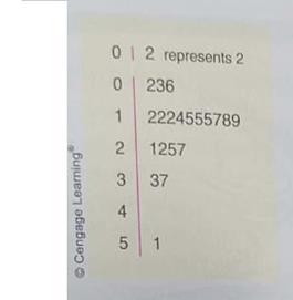
Consider the following random sample of size 20
12 15 21 2 6 3 15 51 22 18
37 12 25 19 33 15 14 17 12 27
A stem-and-leaf display shows that the data are skewed with one outlier.
We can use Minitab to model the bootstrap method for constructing confidence intervals for . (The Professional edition of Minitab is required because of spreadsheet size and other limitations of the Student edition.) This demonstration uses only 1000 samples. Bootstrap uses many thousands.
Step 1 : Create 1000 new samples, each of size 20, by sampling with replacement from the original data. To do this in Minitab, we enter the original 20 data values in column Cl. Then, in column C2, we place equal probabilities of 0.05 beside each of the original data values. Use the menu choices Calc
 Random Data
 Discrete. In the dialogue box, fill in 1000 as the number of rows, store the data in columns C11-C30, and use column C1 for values and column C2 for probabilities.
Step 2 : Find the sample mean of each of the 1000 samples. To do this in Minitab, use the menu choices Calc
 Row Statistics. In the dialogue box, select mean. Use columns C11-C30 as the input variables and store the results in column C31.
Step3 : Order the 1000 means from smallest to largest. In Minitab, use the menu choices Manip Sort. In the dialogue box, indicate C31 as the column to be sorted. Store the results in column C32. Sort by values in column C3I.
Step 4 : Create a 95% confidence interval by finding the boundaries for the middle 95% of the data. In other words, you need to find the values of the 2.5 percentile ( p 2.5 ) and the 97.5 percentile ( P 97. 5 ). Since there are 1000 data values, the 2.5 percentile is the data value in position 25, while the 97.5 percentile is the data value in position 975. The confidence interval is ( p 2.5 ) P 97. 5.
Demonstration Results
Figure 8-9 shows a histogram of the 1000
 values from one bootstrap simulation. Three bootstrap simulations produced the following 95% confidence intervals.
13.90 to 23.90
14.00 to 24.15
14.05 to 23.8
Using the t distribution on the sample data. Minitab produced the interval 13.33 to 24.27. The results of the bootstrap simulations and the t distribution method are quite close.

= r/n in place of p. As discussed in the article "How Much Confidence Should You Have in Binomial Confidence Intervals" appearing in issue no. 45 of the magazine STATS (a publication of the American Statistical Association), use of as an estimate for p means that the actual confidence level for the intervals may in fact be smaller than the specified level c. This problem arises even when n is large, especially if p is not near 1/2.A simple adjustment to the formula for the confidence intervals is the plus four estimate, first suggested by Edwin Bidwell Wilson in 1927. It is also called the Agresti-Coull confidence interval. This adjustment works best for 95% confidence intervals.
The plus four adjustment has us add two successes and two failures to the sample data. This means that r , the number of successes, is increased by 2, and n, the sample size is increased by 4. We use the symbol
, read " P tilde, " for the resulting sample estimate of p. So, = (r + 2)/( n + 4)PROCEDURE
HOW TO COMPUTE A PLUS FOUR CONFIDENCE INTERVAL FOR p
Requirements
Consider a binomial experiment with n trials, where p represents the population probability of success and q = 1 - p represents the population probability of failure. Let r be a random variable that represents the number of successes out of the n binomial trials.
The plus four point estimates for p and q are
The number of trials n should be at least 10.
Approximate confidence interval for p
- E p + E Where
c = confidence level (0 c 1)
z c = critical value for confidence level c based on the standard normal distribution
(a) Consider a random sample of 50 trials with 20 successes. Compute a 95% confidence interval for p using the plus four method.
(b) Compute a traditional 95% confidence interval for p using a random sample of 50 trials with 20 successes.
(c) Compare the lengths of the intervals obtained using the two methods. Is the point estimate closer to 1/2 when using the plus four method Is the margin of error smaller when using the plus four method
Consider the following random sample of size 20
12 15 21 2 6 3 15 51 22 18
37 12 25 19 33 15 14 17 12 27
A stem-and-leaf display shows that the data are skewed with one outlier.
We can use Minitab to model the bootstrap method for constructing confidence intervals for . (The Professional edition of Minitab is required because of spreadsheet size and other limitations of the Student edition.) This demonstration uses only 1000 samples. Bootstrap uses many thousands.
Step 1 : Create 1000 new samples, each of size 20, by sampling with replacement from the original data. To do this in Minitab, we enter the original 20 data values in column Cl. Then, in column C2, we place equal probabilities of 0.05 beside each of the original data values. Use the menu choices Calc
Random Data Discrete. In the dialogue box, fill in 1000 as the number of rows, store the data in columns C11-C30, and use column C1 for values and column C2 for probabilities.Step 2 : Find the sample mean of each of the 1000 samples. To do this in Minitab, use the menu choices Calc
Row Statistics. In the dialogue box, select mean. Use columns C11-C30 as the input variables and store the results in column C31.Step3 : Order the 1000 means from smallest to largest. In Minitab, use the menu choices Manip Sort. In the dialogue box, indicate C31 as the column to be sorted. Store the results in column C32. Sort by values in column C3I.
Step 4 : Create a 95% confidence interval by finding the boundaries for the middle 95% of the data. In other words, you need to find the values of the 2.5 percentile ( p 2.5 ) and the 97.5 percentile ( P 97. 5 ). Since there are 1000 data values, the 2.5 percentile is the data value in position 25, while the 97.5 percentile is the data value in position 975. The confidence interval is ( p 2.5 ) P 97. 5.
Demonstration Results
Figure 8-9 shows a histogram of the 1000
values from one bootstrap simulation. Three bootstrap simulations produced the following 95% confidence intervals.13.90 to 23.90
14.00 to 24.15
14.05 to 23.8
Using the t distribution on the sample data. Minitab produced the interval 13.33 to 24.27. The results of the bootstrap simulations and the t distribution method are quite close.
Explanation Verified
We are introduced to the "plus four" con...
Understanding Basic Statistics 6th Edition by Charles Henry Brase,Corrinne Pellillo Brase
Why don’t you like this exercise?
Other Minimum 8 character and maximum 255 character
Character 255


