
Macroeconomics 1st Edition by Campbell McConnell,Stanley Brue,Sean Flynn
Edition 1ISBN: 978-0077230975Macroeconomics 1st Edition by Campbell McConnell,Stanley Brue,Sean Flynn
Edition 1ISBN: 978-0077230975 Exercise 1
Briefly explain the use of graphs as a way to present economic relationships. What is an inverse relationship How does it graph What is a direct relationship How does it graph Graph and explain the relationships (other things equal) you would expect to find between (a) the number of inches of rainfall per month and the sale of umbrellas, (b) the price of bottled water and the number of bottles sold per year, and (c) the popularity of an entertainer and the price of her concert tickets.
Explanation Verified
Graphs are used extensively in academics and research work due to their instant impression on the reader. A graph can be defined as a visual representation of the data that exhibits a relation between two variables. One of these variables is considered to be influenced by the changes occurring in the other variable.
In Economics, graphs are used widely to express the general relation between variables such as price and quantity, tax rate and tax revenue, etc. In this manner, the relations can be inverse or direct. When the relationship between variable is inverse, a rise in the value of independent variable reduces the value of the dependent variable.
The graph of this relationship is shown as a straight line or a curve that slopes down. This relationship exhibits a situation where the direction of changes in the variables is opposite. In contrast, when the relationship between variable is direct, a rise in the value of independent variable also increases the value of the dependent variable.
The graph of this relation is also shown as a straight line or a curve but in this case it slopes up. This relationship showcases a situation where the direction of changes in the variables is same.
a)
The independent variable is the number of inches of rainfall that occurs in a month. The dependent variable is the sale of umbrellas. When there is a heavy rainfall, people need more umbrellas. Hence, height of rainfall occurred is directly related with sales of umbrella.
This indicates that as number of inches of rainfall increases, the sale of umbrellas is increased. Figure 1 illustrates this relationship between the two variables.
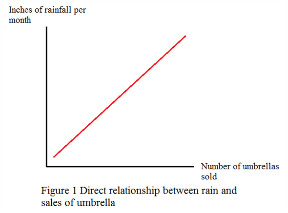 The graph plot shows a straight line that slopes upwards. This is an indication of the fact that a rise in number of inches of rainfall also increases the sale of umbrellas.
Any factor beyond the two described by the graph would bring shifts in the graph. For example, a fall in the income of the consumer will decrease the sales of umbrella irrespective of the intensity of rain.
b)
The independent variable is the price of the bottled water. The dependent variable is the sales of bottles of water. When the price of bottled water is high, consumers are discouraged to buy more bottles. Hence, price of bottled water is inversely related with sales of bottles of water.
Figure 2 illustrates this relationship between the two variables. Note that the graph can also have a curve instead of a straight line, when the relationship between the variables is non-linear.
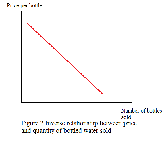 The graph plot shows a straight line that slopes downwards. This is an indication of the fact that a rise in price of bottled water tends to reduce its sale.
Any factor beyond the two described by the graph would bring shifts in the graph. For example, here also, a fall in the income of the consumer will decrease the sales. This will be shown as a leftward shift of the curve. There can be a case when both the quantity and price of bottled water increase simultaneously.
This increase is not disturbing the relationship described because the line showing the inverse relation between price and quantity will remain downward sloping. It is just the fact that there is a favourable change in the demand for bottled water that has increased its demand.
Here, the phrase 'other things equal' matters. When it is said that the price of bottled water is inversely related with sales of bottles of water, all other factors that can influence the sales are assumed unchanged.
However, when there is a change in these factors, say, the arrival of summers, the demand is said to have increased. This will shift the demand to the right, increasing both quantity and price.
c)
The independent variable is popularity of the entertainer. The dependent variable is the price of tickets. When there is a huge popularity of the entertainer, people demand more shows and this increases the price of tickets.
This indicates that as popularity of the entertainer increases, the price of tickets is increased. Figure 1 illustrates this relationship between the two variables.
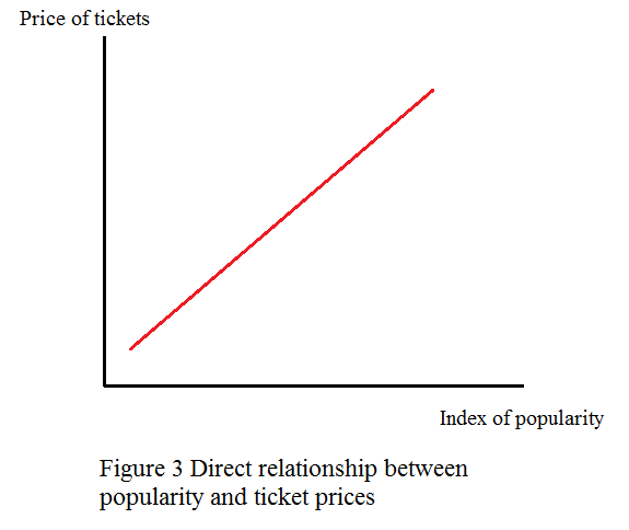 The graph plot shows a straight line that slopes upwards. This illustrates that as the entertainer becomes more famous, her fame also increases the selling price of its tickets.
Any factor beyond the two described by the graph would bring shifts in the graph.
In Economics, graphs are used widely to express the general relation between variables such as price and quantity, tax rate and tax revenue, etc. In this manner, the relations can be inverse or direct. When the relationship between variable is inverse, a rise in the value of independent variable reduces the value of the dependent variable.
The graph of this relationship is shown as a straight line or a curve that slopes down. This relationship exhibits a situation where the direction of changes in the variables is opposite. In contrast, when the relationship between variable is direct, a rise in the value of independent variable also increases the value of the dependent variable.
The graph of this relation is also shown as a straight line or a curve but in this case it slopes up. This relationship showcases a situation where the direction of changes in the variables is same.
a)
The independent variable is the number of inches of rainfall that occurs in a month. The dependent variable is the sale of umbrellas. When there is a heavy rainfall, people need more umbrellas. Hence, height of rainfall occurred is directly related with sales of umbrella.
This indicates that as number of inches of rainfall increases, the sale of umbrellas is increased. Figure 1 illustrates this relationship between the two variables.
The graph plot shows a straight line that slopes upwards. This is an indication of the fact that a rise in number of inches of rainfall also increases the sale of umbrellas. Any factor beyond the two described by the graph would bring shifts in the graph. For example, a fall in the income of the consumer will decrease the sales of umbrella irrespective of the intensity of rain.
b)
The independent variable is the price of the bottled water. The dependent variable is the sales of bottles of water. When the price of bottled water is high, consumers are discouraged to buy more bottles. Hence, price of bottled water is inversely related with sales of bottles of water.
Figure 2 illustrates this relationship between the two variables. Note that the graph can also have a curve instead of a straight line, when the relationship between the variables is non-linear.
The graph plot shows a straight line that slopes downwards. This is an indication of the fact that a rise in price of bottled water tends to reduce its sale. Any factor beyond the two described by the graph would bring shifts in the graph. For example, here also, a fall in the income of the consumer will decrease the sales. This will be shown as a leftward shift of the curve. There can be a case when both the quantity and price of bottled water increase simultaneously.
This increase is not disturbing the relationship described because the line showing the inverse relation between price and quantity will remain downward sloping. It is just the fact that there is a favourable change in the demand for bottled water that has increased its demand.
Here, the phrase 'other things equal' matters. When it is said that the price of bottled water is inversely related with sales of bottles of water, all other factors that can influence the sales are assumed unchanged.
However, when there is a change in these factors, say, the arrival of summers, the demand is said to have increased. This will shift the demand to the right, increasing both quantity and price.
c)
The independent variable is popularity of the entertainer. The dependent variable is the price of tickets. When there is a huge popularity of the entertainer, people demand more shows and this increases the price of tickets.
This indicates that as popularity of the entertainer increases, the price of tickets is increased. Figure 1 illustrates this relationship between the two variables.
The graph plot shows a straight line that slopes upwards. This illustrates that as the entertainer becomes more famous, her fame also increases the selling price of its tickets. Any factor beyond the two described by the graph would bring shifts in the graph.
Macroeconomics 1st Edition by Campbell McConnell,Stanley Brue,Sean Flynn
Why don’t you like this exercise?
Other Minimum 8 character and maximum 255 character
Character 255


