Business Forecasting 9th Edition by John Hanke, Dean Wichern

Exercise 4

TUX
John Mosby, owner of several Mr. Tux rental stores, is beginning to forecast his most important business variable, monthly dollar sales (see the Mr. Tux cases in previous chapters). One of his employees, Virginia Perot, gathered the sales data shown in Case 2-2. John now wants to create a forecast based on these sales data using moving average and exponential smoothing techniques.
John used Minitab in Case 3-2 to determine that these data are both trending and seasonal. He has been told that simple moving averages and exponential smoothing techniques will not work with these data but decides to find out for himself.
He begins by trying a three-month moving average. The program calculates several summary forecast error measurements. These values summarize the errors found in predicting actual historical data values using a three-month moving average. John decides to record two of these error measurements:

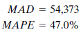
The MAD (mean absolute deviation) is the average absolute error made in forecasting past values. Each forecast using the three-month moving average method is off by an average of 54,373. The MAPE (mean absolute percentage error) shows the error as a percentage of the actual value to be forecast. The average error using the three-month moving average technique is 47%, or almost half as large as the value to be forecast.
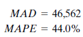
Next, John tries simple exponential smoothing. The program asks him to input the smoothing constant ( ? ) to be used or to ask that the optimum ? value be calculated. John does the latter, and the program finds the optimum ? value to be.867. Again he records the appropriate error measurements:

John asks the program to use Holt's linear exponential smoothing on his data. This program uses the exponential smoothing method but can account for a trend in the data as well. John has the program use a smoothing constant of.4 for both ? and ?. The two summary error measurements for Holt's method are

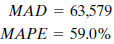
John is surprised to find larger measurement errors for this technique. He decides that the seasonal aspect of the data is the problem. Winters' multiplicative exponential smoothing is the next method John tries. This method can account for seasonal factors as well as trend. John uses smoothing constants of ? =.2, ? =.2, and ? =.2. Error measurements are

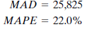
When John sits down and begins studying the results of his analysis, he is disappointed. The Winters' method is a big improvement; however, the MAPE is still 22%. He had hoped that one of the methods he used would result in accurate forecasts of past periods; he could then use this method to forecast the sales levels for coming months over the next year. But the average absolute errors (MADs) and percentage errors ( MAPE s) for these methods lead him to look for another way of forecasting.
Although not calculated directly in Minitab, the MPE (mean percentage error) measures forecast bias. What is the ideal value for the MPE ? What is the implication of a negative sign on the MPE ?