Business Forecasting 9th Edition by John Hanke, Dean Wichern

Exercise 5

BUSINESS ACTIVITY INDEX FOR SPOKANE COUNTY
Prior to 1973, Spokane County, Washington, had no up-to-date measurement of general business activity. What happens in this area as a whole, however, affects every local business, government agency, and individual. Plans and policies made by an economic unit would be incomplete without some reliable knowledge about the recent performance of the economy of which the unit is a component part. A Spokane business activity index should serve as a vital input in the formulation of strategies and decisions in private as well as in public organizations.
A business activity index is an indicator of the relative changes in overall business conditions within a specified region. At the national level, the gross domestic product (GDP, computed by the Department of Commerce) and the industrial production index (compiled by the Federal Reserve Board) are generally considered excellent indicators. Each of these series is based on thousands of pieces of information-the collecting, editing, and computing of which are costly and time-consuming undertakings. For a local area such as Spokane County, Washington, a simplified version, capable of providing reasonably accurate and current information at moderate cost, is very desirable.
Multiple regression can be used to construct a business activity index. There are three essential questions that must be answered in order to construct such an index:
• What are the components of the index?
• Do these components adequately represent the changes in overall business conditions?
• What weight should be assigned to each of the chosen components?
Answers to these questions can be obtained through regression analysis.
Dr. Shik Chun Young, professor of economics at Eastern Washington University, is attempting to develop a business activity index for Spokane County. Young selects personal income as the dependent variable. At the county level, personal income is judged as the best available indicator of local business conditions. Personal income measures the total income received by households before personal taxes are paid. Since productive activities are typically remunerated by monetary means, personal income may indeed be viewed as a reasonable proxy for the general economic performance. Why then is it necessary to construct another index if personal income can serve as a good business activity indicator? Unfortunately, personal income data at the county level are estimated by the U.S. Department of Commerce on an annual basis and are released 16 months too late. Consequently, these data are of little use for short-term planning. Young's task is to establish an up-to-date business activity index.
The independent variables are drawn from those local data that are readily available on a monthly basis. Currently, about 50 series of such monthly data are available, ranging from employment, bank activities, and real estate transactions to electrical consumption. If each series were to be included in the regression analysis, the effort would not be very productive because only a handful of these series would likely be statistically significant. Therefore, some knowledge of the relationship between personal income and the available data is necessary in order to determine which independent variables are to be included in the regression equation. From Young's knowledge of the Spokane economy, the following 10 series are selected:
X 1 , total employment
X 2 , manufacturing employment
X 3 , construction employment
X 4 , wholesale and retail trade employment
X 5 , service employment
X 6 , bank debits
X 7 , bank demand deposits
X 8 , building permits issued
X 9 , real estate mortgages
X 10 , total electrical consumption
The first step in the analysis is to fit the model
E ( Y ) = ? 0 + ? 1 X 1 + ? 2 X 2 +…+ ? 10 X 10
where

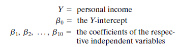
When the preceding model is fit to the data, the adjusted
is.96, which means that the 10 variables used together explain 96% of the variability in the dependent variable, personal income. However, other regression statistics indicate problems. First, of these 10 independent variables, only three-namely, total employment, service employment, and bank debits-have a computed t value significant at the.05 level. Second, the correlation matrix shows a high degree of interdependence among several of the independent variables-multicollinearity. 21 For example, total employment and bank debits have a correlation coefficient of.88; total electrical consumption and bank demand deposits,.76; and building permits issued and real estate mortgages,.68. Third, a test for autocorrelation using the DurbinWatson statistic of.91 indicates that successive values of the dependent variable are positively correlated. Of course, autocorrelation is rather common in time series data; in general, observations in the same series tend to be related to one another.
Since one of the basic assumptions in regression analysis is that the observations of the dependent variable are random, Young chooses to deal with the autocorrelation problem first. He decides to calculate first differences, or changes, in an attempt to minimize the interdependence among the observations in each of the time series. The 10 independent variables are now measured by the difference between the periods rather than by the absolute value for each period. So that the sets of data can be distinguished, a new designation for the independent variables is used:
? X 1 , change in total employment
? X 2 , change in manufacturing employment
? X 3 , change in construction employment
? X 4 , change in wholesale and retail trade employment
? X 5 , change in service employment
? X 6 , change in bank debits
? X 7 , change in demand deposits
? X 8 , change in building permits issued
? X 9 , change in real estate mortgages
? X 10 , change in total electrical consumption
The regression model becomes
E (? Y ) = ? 0 + ? 1 ? X 1 + ? 2 ? X 2 +…+ ? 10 ? X 10
where

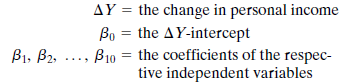
A regression run using this model, based on the first difference data, produces a Durbin-Watson statistic of 1.71. It indicates that no serious autocorrelation remains.
The next step is to determine which of the 10 variables are significant predictors of the dependent variable. The dependent variable, ? Y , is regressed against several possible combinations of the 10 potential predictors in order to select the best equation. The criteria used in the selection are
• A satisfactorily high

• Low correlation coefficients among the independent variables
• Significant (at the.05 level) coefficients for each of the independent variables
After careful scrutiny of the regression results, Young finds that the equation that contains ? X 4 , ? X 5 , and ? X 10 as independent variables best meets the foregoing criteria.
However, Young reasons that (in addition to commercial and industrial uses) total electrical consumption includes residential consumption, which should not have a significant relation to business activity in the near term. To test this hypothesis, Young subdivides the total electrical consumption into four variables:
? X 11 , change in residential electricity use
? X 12 , change in commercial electricity use
? X 13 , change in industrial electricity use
? X 14 , change in commercial and industrial electricity use
All four variables, combined with ? X 4 and ? X 5 , are used to produce four new regression equations (see Table 8-12).
Statistical analysis indicates that Equation D in Table 8-12 is the best. Compared with the previous equation, which contained ? X 4 , ? X 5 , and ? X 10 as independent variables, Equation A is the only one that shows a deterioration in statistical significance. This result confirms Young's notion that commercial and industrial electricity uses are better predictors of personal income than total electrical consumption, which includes residential electricity use.
Therefore, Equation D is selected as the final regression equation, and the results are

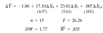
The figures in parentheses below the regression coefficients are the standard errors of the estimated coefficients. The t values of the coefficients are 4.20, 4.10, and 3.50 for ? X 4 , ? X 5 , and ? X 14 , respectively. The R 2 indicates that nearly 84% of the variance in change in personal income is explained by the three independent variables. The Durbin-Watson (DW) statistic shows that autocorrelation is not a problem. In addition, the correlation coefficient matrix of Table 8-13 demonstrates a low level of interdependence among the three independent variables.
For index construction purposes, the independent variables in the final regression equation become the index components. The weights of the components can be determined from the regression coefficients.
(Recall that the regression coefficient represents the average change in the dependent variable for a one-unit increase in the independent variable.) However, because the variables in the regression equation are not measured in the same units (for example, ? Y is measured in thousands of dollars and ? X 14 in thousands of kilowatt-hours), the regression coefficients must be transformed into relative values. This transformation is accomplished by computing their standardized or B coefficients.

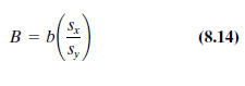
where

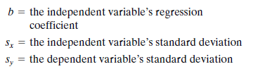
The values of all these statistics are typically available from the regression computer output. Hence, the standardized coefficients of the three independent variables are

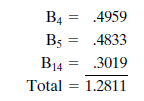
Because the sum of the weights in an index must be 100%, the standardized coefficients are normalized as shown in Table 8-14.
After the components and their respective weights have been determined, the following steps give the index:
1. Compute the percentage change of each component since the base period.
2. Multiply the percentage change by the appropriate weight.
3. Sum the weighted percentage changes obtained in step 2.
The completed Spokane County activity index, for the time period considered, is compared with the
U.S. GNP, in constant dollars (1967 = 100), in Figure 8-12.
TABLE 8-12 Young's Regression Variables

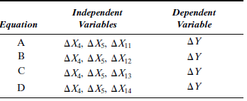
TABLE 8-13 Correlation Coefficient Matrix

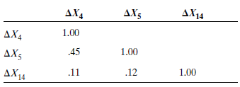
FIGURE 8-12 Spokane County Business Activity Index and the U.S. GNP, in Constant Dollars ( 1967 = 100 )

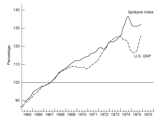
TABLE 8-14 Standardized Coefficients

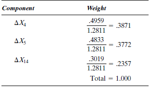
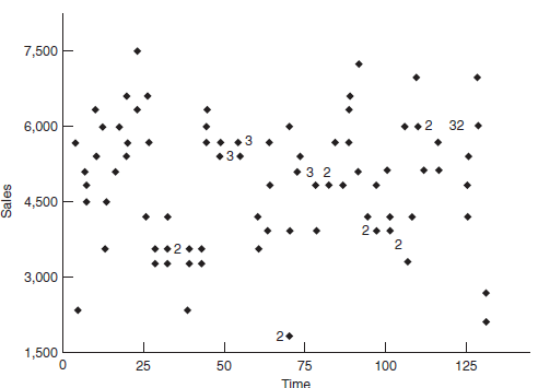
FIGURE 8-13 Restaurant Sales, January 1981-December 1982

Is there any potential for the use of lagged data?