
Microeconomics 6th Edition by Robert Hall, Shirley Kuiper, Marc Lieberman
Edition 6ISBN: 978-1133708735Microeconomics 6th Edition by Robert Hall, Shirley Kuiper, Marc Lieberman
Edition 6ISBN: 978-1133708735 Exercise 3
Figure 1 shows the market for gasoline with a negative externality from pollution. Using the information in Figures 1 and 2,calculate the dollar value of the deadweight loss per period before any government intervention.
Figure 1 Inefficiency from a Negative Externality
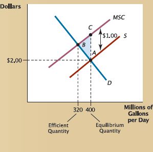
In the competitive market for gasoline,the market equilibrium is at point A with quantity at 400 million. But the supply curve includes only marginal costs to private suppliers,ignoring the negative externality of $1.00 per gallon. When the negative externality is added to other costs,the result is the marginal social cost curve ( MSC ). The efficient output level (320 million)is at point B. Without government intervention,the units from 320 million to 400 million are produced,even though their full cost (given by the MSC curve)is greater than their value (on the demand curve). The result is a deadweight loss equal to the area of the shaded triangle.
Figure 2 A Tax on Producers to Correct a Negative Externality
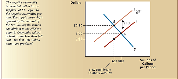
Figure 1 Inefficiency from a Negative Externality
In the competitive market for gasoline,the market equilibrium is at point A with quantity at 400 million. But the supply curve includes only marginal costs to private suppliers,ignoring the negative externality of $1.00 per gallon. When the negative externality is added to other costs,the result is the marginal social cost curve ( MSC ). The efficient output level (320 million)is at point B. Without government intervention,the units from 320 million to 400 million are produced,even though their full cost (given by the MSC curve)is greater than their value (on the demand curve). The result is a deadweight loss equal to the area of the shaded triangle.
Figure 2 A Tax on Producers to Correct a Negative Externality
Explanation Verified
Having the figure (3)into mind,the trian...
Microeconomics 6th Edition by Robert Hall, Shirley Kuiper, Marc Lieberman
Why don’t you like this exercise?
Other Minimum 8 character and maximum 255 character
Character 255


