An Introduction to Management Science 13th Edition by David Anderson,Dennis Sweeney ,Thomas Williams ,Jeffrey Camm, Kipp Martin
Edition 13ISBN: 978-1439043271An Introduction to Management Science 13th Edition by David Anderson,Dennis Sweeney ,Thomas Williams ,Jeffrey Camm, Kipp Martin
Edition 13ISBN: 978-1439043271 Exercise 30
Reiser Sports wants to determine the number of All-Pro (A) and College (C) footballs to produce in order to maximize profit over the next four-week planning horizon. Constraints affecting the production quantities are the production capacities in three departments: cutting and dyeing; sewing; and inspection and packaging. For the four-week planning period, 340 hours of cutting and dyeing time, 420 hours of sewing time, and 200 hours of inspection and packaging time are available. All-Pro footballs provide a profit of $5 per unit and College footballs provide a profit of $4 per unit. The linear programming model with production times expressed in minutes is as follows: 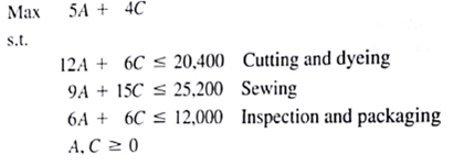
A portion of the graphical solution to the Reiser problem is shown in Figure 2.23.
a. Shade the feasible region for this problem.
b. Determine the coordinates of each extreme point and the corresponding profit. Which extreme point generates the highest profit?
c. Draw the profit line corresponding to a profit of $4000. Move the profit line as far from the origin as you can in order to determine which extreme point will provide the optimal solution. Compare your answer with the approach you used in part (b).
d. Which constraints are binding? Explain.
e. Suppose that the values of the objective function coefficients are $4 for each All-Pro model produced and $5 for each College model. Use the graphical solution procedure to determine the new optimal solution and the corresponding value of profit.
FIGURE 2.22 GRAPH OF THE CONSTRAINT LINES FOR EXERCISE 21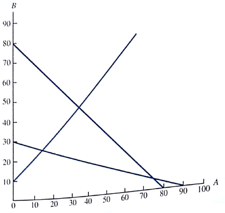
FIGURE 2.23 PORTION OF THE GRAPHICAL SOLUTION FOR EXERCISE 22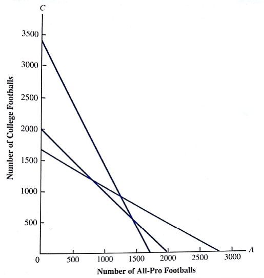
Explanation Verified
Linear programming:
Linear programming ...
An Introduction to Management Science 13th Edition by David Anderson,Dennis Sweeney ,Thomas Williams ,Jeffrey Camm, Kipp Martin
Why don’t you like this exercise?
Other Minimum 8 character and maximum 255 character
Character 255


