An Introduction to Management Science 13th Edition by David Anderson,Dennis Sweeney ,Thomas Williams ,Jeffrey Camm, Kipp Martin

Exercise 29

Air pollution control specialists in southern California monitor the amount of ozone, carbon dioxide, and nitrogen dioxide in the air on an hourly basis. The hourly time series data exhibit seasonally, with the levels of pollutants showing patterns that vary over the hours in the day. On July 15, 16, and 17, the following levels of nitrogen dioxide were observed for the 12 hours from 6:00 A.M. to 6:00 P.M.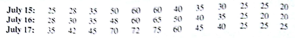
a. Construct a time series plot. What type of pattern exits in the data?
b. Use an Excel or LINGO model with dummy variables as follow to develop an equation to account for seasonal effects in the data: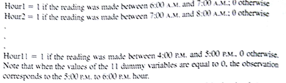
c. Using the equation developed in part (b) compute estimates of the levels of nitrogen dioxide for July 18.
d. Let t = 1 to refer to the observation in hour 1 on July 15; t = 2 to refer to the observation in hour 2 of year 15;... and t = 36 to refer to the observation in hour 12 of July 17. Using the dummy variables defined in part (b) and rs , develop an equation to account for seasonal effects and any linear trend in the time series. Based upon the seasonal effects in the data and linear trend, compute estimates of the levels of nitrogen dioxide for July 18.