Campbell Biology 11th Edition by Lisa Urry,Michael Cain,Steven Wasserman,Peter Minorsky,Jane Reece

Exercise 1

Are Two Genes Linked or Unlinked Genes that are in close proximity on the same chromosome will result in the linked alleles being inherited together more often than not. But how can you tell if certain alleles are inherited together due to linkage or whether they just happen to assort together In this exercise, you will use a simple statistical test, the chi-square ( 2) test, to analyze phenotypes of F1 testcross progeny in order to see whether two genes are linked or unlinked.
How These Experiments Are Done If genes are unlinked and assorting independently, the phenotypic ratio of offspring from an F1 testcross is expected to be 1:1:1:1 (see Figure 12.9). If the two genes are linked, however, the observed phenotypic ratio of the offspring will not match the expected ratio. Given random fluctuations in the data, how much must the observed numbers deviate from the expected numbers for us to conclude that the genes are not assorting independently but may instead be linked To answer this question, scientists use a statistical test called a chi-square ( 2) test. This test compares an observed data set to an expected data set predicted by a hypothesis (here, that the genes are unlinked) and measures the discrepancy between the two, thus determining the "goodness of fit." If the discrepancy between the observed and expected data sets is so large that it is unlikely to have occurred by random fluctuation, we say there is statistically significant evidence against the hypothesis (or, more specifically, evidence for the genes being linked). If the discrepancy is small, then our observations are well explained by random variation alone. In this case, we say the observed data are consistent with our hypothesis, or that the discrepancy is statistically insignificant. Note, however, that consistency with our hypothesis is not the same as proof of our hypothesis. Also, the size of the experimental data set is important: With small data sets like this one, even if the genes are linked, discrepancies might be small by chance alone if the linkage is weak. (For simplicity, we overlook the effect of sample size here.)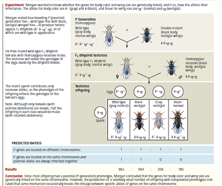
Data from the Simulated Experiment In cosmos plants, purple stem ( A ) is dominant to green stem ( a ), and short petals ( B ) is dominant to long petals ( b ). In a simulated cross, AABB plants were crossed with aabb plants to generate F1 dihybrids ( AaBb ), which were then test crossed ( AaBb × aabb ). A total of 900 offspring plants were scored for stem color and flower petal length.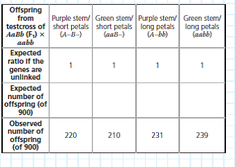
The 2 value means nothing on its own-it is used to find the probability that, assuming the hypothesis is true, the observed data set could have resulted from random fluctuations. A low probability suggests the observed data are not consistent with the hypothesis, and thus the hypothesis should be rejected. A standard cut-off point used by biologists is a probability of 0.05 (5%). If the probability corresponding to the 2 value is 0.05 or less, the differences between observed and expected values are considered statistically significant and the hypothesis (that the genes are unlinked) should be rejected. If the probability is above 0.05, the results are not statistically significant; the observed data is consistent with the hypothesis. To find the probability, locate your 2 value in the 2 Distribution Table in Appendix F. The "degrees of freedom" (df) of your data set is the number of categories (here, 4 phenotypes)minus 1, so df = 3. (a) Determine which values on the df = 3 line of the table your calculated 2 value lies between. (b) The column headings for these values show the probability range for your 2 number. Based on whether there are nonsignificant ( p 0.05) or significant ( p 0.05) differences between the observed and expected values, are the data consistent with the hypothesis that the two genes are unlinked and assorting independently, or is there enough evidence to reject this hypothesis