Essentials of Business Analytics 1st Edition by Jeffrey Camm,James Cochran,Michael Fry,Jeffrey Ohlmann ,David Anderson

Exercise 9

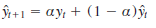
Many forecasting models use parameters that are estimated using nonlinear optimization. A good example is the Bass model introduced in this chapter. Another example is the exponential smoothing forecasting model discussed in Chapter 5. The exponential smoothing model is common in practice and is described in further detail in Chapter 5. For
instance, the basic exponential smoothing model for forecasting sales is

Where

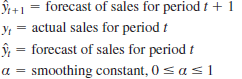
This model is used recursively; the forecast for time period t 1 1 is based on the forecast for period t,
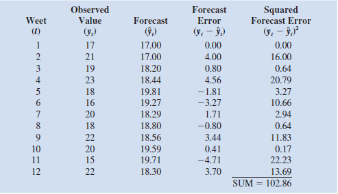
, the observed value of sales in period t , y t , and the smoothing parameter _. The use of this model to forecast sales for 12 months is illustrated in the following table with the smoothing constant _ 5 0.3. The forecast errors,
, are calculated in the fourth column. The value of _ is often chosen by minimizing the sum of squared forecast errors. The last column of the table shows the square of the forecast error and the sum of squared forecast errors. In using exponential smoothing models, one tries to choose the value of _ that provides the best forecasts.
a. The file ExpSmooth contains the observed data shown here. Construct this table using the formula above. Note that we set the forecast in period 1 to the observed in period 1 to get started
= 17 then the formula above for
is used starting in period 2. Make sure to have a single cell corresponding to _ in your spreadsheet model. After confirming the values in the table below with _ 5 0.3, try different values of _ to see if you can get a smaller sum of squared forecast errors.
b. Use Excel Solver to find the value of _ that minimizes the sum of squared forecast errors.