Deck 9: Regression Analysis
Full screen (f)
Question
Question
Question
Question
Question
Question
Question
Question
Question
Question
Question
Question
Question
Question
Question
Question
Question
Question
Question
Question
Question
Question
Question
Question
Question
Question
Question
Question
Question
Question
Question
Question
Question
Question
Question
Question
Question
Question
Question
Question
Question
Exhibit 9.1
The following questions are based on the problem description and spreadsheet below.
A company has built a regression model to predict the number of labor hours (Yi) required to process a batch of parts (Xi). It has developed the following Excel spreadsheet of the results.

Refer to Exhibit 9.1. Provide a rough 95% confidence interval on the number of labor hours for a batch of 5 parts.
The following questions are based on the problem description and spreadsheet below.
A company has built a regression model to predict the number of labor hours (Yi) required to process a batch of parts (Xi). It has developed the following Excel spreadsheet of the results.
Refer to Exhibit 9.1. Provide a rough 95% confidence interval on the number of labor hours for a batch of 5 parts.
Question
The company would like to build a prediction interval on the pressure for a can with a temperature of 125 degrees. What formula should be entered in cells B17:F21 of the following spreadsheet to compute this prediction interval? Partial results of the Regression analysis of the data are provided below.

Question
Exhibit 9.2
The following questions are based on the problem description and spreadsheet below.
A paint manufacturer is interested in knowing how much pressure (in pounds per square inch, PSI) builds up inside aerosol cans at various temperatures (degrees Fahrenheit). It has developed the following Excel spreadsheet of the results.

Refer to Exhibit 9.2. Interpret the meaning of the "Lower 95%" and "Upper 95%" terms in cells F16:G16 of the spreadsheet.
The following questions are based on the problem description and spreadsheet below.
A paint manufacturer is interested in knowing how much pressure (in pounds per square inch, PSI) builds up inside aerosol cans at various temperatures (degrees Fahrenheit). It has developed the following Excel spreadsheet of the results.
Refer to Exhibit 9.2. Interpret the meaning of the "Lower 95%" and "Upper 95%" terms in cells F16:G16 of the spreadsheet.
Question
Exhibit 9.2
The following questions are based on the problem description and spreadsheet below.
A paint manufacturer is interested in knowing how much pressure (in pounds per square inch, PSI) builds up inside aerosol cans at various temperatures (degrees Fahrenheit). It has developed the following Excel spreadsheet of the results.
Refer to Exhibit 9.2. What is the estimated regression function for this problem? Explain what the terms in your equation mean.
Question
Exhibit 9.1
The following questions are based on the problem description and spreadsheet below.
A company has built a regression model to predict the number of labor hours (Yi) required to process a batch of parts (Xi). It has developed the following Excel spreadsheet of the results.
Refer to Exhibit 9.1. Interpret the meaning of the "Lower 95%" and "Upper 95%" terms in cells F16:G16 of the spreadsheet.
Question
Exhibit 9.1
The following questions are based on the problem description and spreadsheet below.
A company has built a regression model to predict the number of labor hours (Yi) required to process a batch of parts (Xi). It has developed the following Excel spreadsheet of the results.
Refer to Exhibit 9.1. Interpret the meaning of R Square in cell B3 of the spreadsheet.
Question
Question
Exhibit 9.3
The following questions are based on the problem description and spreadsheet below.
A researcher is interested in determining how many calories young men consume. She measured the age of the individuals and recorded how much food they ate each day for a month. The average daily consumption was recorded as the dependent variable. She has developed the following Excel spreadsheet of the results.

Refer to Exhibit 9.3. What is the estimated regression function for this problem? Explain what the terms in your equation mean
The following questions are based on the problem description and spreadsheet below.
A researcher is interested in determining how many calories young men consume. She measured the age of the individuals and recorded how much food they ate each day for a month. The average daily consumption was recorded as the dependent variable. She has developed the following Excel spreadsheet of the results.
Refer to Exhibit 9.3. What is the estimated regression function for this problem? Explain what the terms in your equation mean
Question
Exhibit 9.1
The following questions are based on the problem description and spreadsheet below.
A company has built a regression model to predict the number of labor hours (Yi) required to process a batch of parts (Xi). It has developed the following Excel spreadsheet of the results.
Refer to Exhibit 9.1. What is the estimated regression function for this problem? Explain what the terms in your equation mean.
Question
The company would like to build a prediction interval on the time for a new batch of 8 parts. What formula should be entered in cells B17:F21 of the following spreadsheet to compute this prediction interval? Partial results of the Regression analysis of the data are provided below.

Question
Exhibit 9.2
The following questions are based on the problem description and spreadsheet below.
A paint manufacturer is interested in knowing how much pressure (in pounds per square inch, PSI) builds up inside aerosol cans at various temperatures (degrees Fahrenheit). It has developed the following Excel spreadsheet of the results.
Refer to Exhibit 9.2. Test the significance of the model and explain which values you used to reach your conclusions.
Question
Question
Exhibit 9.1
The following questions are based on the problem description and spreadsheet below.
A company has built a regression model to predict the number of labor hours (Yi) required to process a batch of parts (Xi). It has developed the following Excel spreadsheet of the results.
Refer to Exhibit 9.1. Test the significance of the model and explain which values you used to reach your conclusions.
Question
Exhibit 9.1
The following questions are based on the problem description and spreadsheet below.
A company has built a regression model to predict the number of labor hours (Yi) required to process a batch of parts (Xi). It has developed the following Excel spreadsheet of the results.
Refer to Exhibit 9.1. Predict the mean number of labor hours for a batch of 5 parts.
Question
Exhibit 9.2
The following questions are based on the problem description and spreadsheet below.
A paint manufacturer is interested in knowing how much pressure (in pounds per square inch, PSI) builds up inside aerosol cans at various temperatures (degrees Fahrenheit). It has developed the following Excel spreadsheet of the results.
Refer to Exhibit 9.2. Predict the mean pressure for a temperature of 120 degrees.
Question
Exhibit 9.2
The following questions are based on the problem description and spreadsheet below.
A paint manufacturer is interested in knowing how much pressure (in pounds per square inch, PSI) builds up inside aerosol cans at various temperatures (degrees Fahrenheit). It has developed the following Excel spreadsheet of the results.
Refer to Exhibit 9.2. Interpret the meaning of R Square in cell B3 of the spreadsheet.
Question
Question
Question
Question
Question
Exhibit 9.5
The following questions are based on the description and spreadsheet below.
An analyst has identified 3 independent variables (X1, X2,X3) which might be used to predict Y. He has computed the regression equations using all of the variables and the results are summarized in the following table.

Refer to Exhibit 9.5. Based on the data in the table which is the best model for the charity to use? Explain which values you used to reach your conclusion.
The following questions are based on the description and spreadsheet below.
An analyst has identified 3 independent variables (X1, X2,X3) which might be used to predict Y. He has computed the regression equations using all of the variables and the results are summarized in the following table.
Refer to Exhibit 9.5. Based on the data in the table which is the best model for the charity to use? Explain which values you used to reach your conclusion.
Question
Exhibit 9.5
The following questions are based on the description and spreadsheet below.
An analyst has identified 3 independent variables (X1, X2,X3) which might be used to predict Y. He has computed the regression equations using all of the variables and the results are summarized in the following table.
Refer to Exhibit 9.5. Predict the mean value based on (X1, X2, X3) = (3, 32, 50). Use the best predictive model based on data from the table.
Question
Exhibit 9.4
The following questions are based on the problem description and spreadsheet below.
A charitable organization wants to determine what type of people donate to charities like itself. The charity felt that a person's education (in years), annual income, ($1,000) and the number of children the person had were important variables to consider. The charity developed regression models for all of the possible combinations of these three variables but does not know what to do with the results.

Refer to Exhibit 9.4. Predict the mean donation by a person with 16 years of education, $90,000 annual income and 2 children. Use a full model based on data from the table.
The following questions are based on the problem description and spreadsheet below.
A charitable organization wants to determine what type of people donate to charities like itself. The charity felt that a person's education (in years), annual income, ($1,000) and the number of children the person had were important variables to consider. The charity developed regression models for all of the possible combinations of these three variables but does not know what to do with the results.
Refer to Exhibit 9.4. Predict the mean donation by a person with 16 years of education, $90,000 annual income and 2 children. Use a full model based on data from the table.
Question
Question
Exhibit 9.7
The partial regression output below applies to the following questions.

Refer to Exhibit 9.7. What is the SS for Total?
The partial regression output below applies to the following questions.
Refer to Exhibit 9.7. What is the SS for Total?
Question
Exhibit 9.6
The partial regression output below applies to the following questions.

Refer to Exhibit 9.6. What is the F-statistic value?
The partial regression output below applies to the following questions.
Refer to Exhibit 9.6. What is the F-statistic value?
Question
Exhibit 9.7
The partial regression output below applies to the following questions.
Refer to Exhibit 9.7. What is the SS for Residual and MS for Residual?
The partial regression output below applies to the following questions.
Refer to Exhibit 9.7. What is the SS for Residual and MS for Residual?
Question
Assume you have chosen to use all three variables in your model. Test the significance of the model and explain which values you used to reach your conclusion.

Question
Exhibit 9.3
The following questions are based on the problem description and spreadsheet below.
A researcher is interested in determining how many calories young men consume. She measured the age of the individuals and recorded how much food they ate each day for a month. The average daily consumption was recorded as the dependent variable. She has developed the following Excel spreadsheet of the results.
Refer to Exhibit 9.3. Test the significance of the model and explain which values you used to reach your conclusions.
Question
Exhibit 9.4
The following questions are based on the problem description and spreadsheet below.
A charitable organization wants to determine what type of people donate to charities like itself. The charity felt that a person's education (in years), annual income, ($1,000) and the number of children the person had were important variables to consider. The charity developed regression models for all of the possible combinations of these three variables but does not know what to do with the results.
Refer to Exhibit 9.4. Based on the data in the table which is the best model for the charity to use? Explain which values you used to reach your conclusion.
Question
Exhibit 9.3
The following questions are based on the problem description and spreadsheet below.
A researcher is interested in determining how many calories young men consume. She measured the age of the individuals and recorded how much food they ate each day for a month. The average daily consumption was recorded as the dependent variable. She has developed the following Excel spreadsheet of the results.
Refer to Exhibit 9.3. Interpret the meaning of the "Lower 95%" and "Upper 95%" terms in cells F16:G16 of the spreadsheet.
Question
The researcher would like to build a prediction interval on the calories consumed by an 18 year old man. What formula should be entered in cells B17:F21 of the following spreadsheet to compute this prediction interval? Partial results of the Regression analysis of the data are provided below.

Question
Exhibit 9.3
The following questions are based on the problem description and spreadsheet below.
A researcher is interested in determining how many calories young men consume. She measured the age of the individuals and recorded how much food they ate each day for a month. The average daily consumption was recorded as the dependent variable. She has developed the following Excel spreadsheet of the results.
Refer to Exhibit 9.3. Interpret the meaning of R square in cell B3 of the spreadsheet.
Question
Project 9.1 - Test Stand Cost Analysis Estimation
Handel Manufacturing produces test stands for various maintenance functions ranging from automobile to jet airline testing stations. For years, their cost estimating function was based on a myriad of historical data fed into a cost analysis model that produced very accurate estimates of both development and support costs for various proposed test stands. James Mudd was a recent hire into the cost analysis shop. Unfortunately, during his first week on the job, James deleted the cost analysis database and failed to maintain a backup of the model. Fortunately, all is not lost. The computer support personnel can come in Monday and retrieve the model using their system backup tapes. Unfortunately, the cost proposals for three new test stand development and deployment projects are due first thing Monday morning. Since James recently left the company, you have been tasked to complete the cost estimate portion of the proposals.
After much gnashing of your teeth, you settle down to make the best of what you initially believe is a losing situation. While studying James' files you find historical records on 25 recent test stand development and deployment projects. Rejuvenated, you realize you can succeed in this prematurely perceived doomed situation. All you need to do is analyze this historical data, develop some cost estimating functions using regression, and then use your regression models to develop estimates for the three projects due Monday. The historical data in the files is the following.
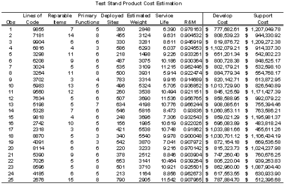 The data estimates for the three cost proposal due Monday is the following:
One thing unclear from reading the files was on the form of the cost estimating relationships contained within the lost cost analysis model. You are somewhat sure the regression models were not polynomial in form, but you are not certain of this fact. You are not even sure which variables were included in the model for development cost and which variables were included in the model for support costs. However, you are undaunted because you know you can develop accurate models and produce good cost estimates for each of the proposed projects.
Develop appropriate models for development and for support costs. Use these models to develop cost estimates for each of the new lines of test stands. For each of these cost estimates provide 95% confidence intervals for the predicted values.
Handel Manufacturing produces test stands for various maintenance functions ranging from automobile to jet airline testing stations. For years, their cost estimating function was based on a myriad of historical data fed into a cost analysis model that produced very accurate estimates of both development and support costs for various proposed test stands. James Mudd was a recent hire into the cost analysis shop. Unfortunately, during his first week on the job, James deleted the cost analysis database and failed to maintain a backup of the model. Fortunately, all is not lost. The computer support personnel can come in Monday and retrieve the model using their system backup tapes. Unfortunately, the cost proposals for three new test stand development and deployment projects are due first thing Monday morning. Since James recently left the company, you have been tasked to complete the cost estimate portion of the proposals.
After much gnashing of your teeth, you settle down to make the best of what you initially believe is a losing situation. While studying James' files you find historical records on 25 recent test stand development and deployment projects. Rejuvenated, you realize you can succeed in this prematurely perceived doomed situation. All you need to do is analyze this historical data, develop some cost estimating functions using regression, and then use your regression models to develop estimates for the three projects due Monday. The historical data in the files is the following.
The data estimates for the three cost proposal due Monday is the following:One thing unclear from reading the files was on the form of the cost estimating relationships contained within the lost cost analysis model. You are somewhat sure the regression models were not polynomial in form, but you are not certain of this fact. You are not even sure which variables were included in the model for development cost and which variables were included in the model for support costs. However, you are undaunted because you know you can develop accurate models and produce good cost estimates for each of the proposed projects.
Develop appropriate models for development and for support costs. Use these models to develop cost estimates for each of the new lines of test stands. For each of these cost estimates provide 95% confidence intervals for the predicted values.
Question
Exhibit 9.6
The partial regression output below applies to the following questions.
Refer to Exhibit 9.6. What is the MS for Residual?
The partial regression output below applies to the following questions.
Refer to Exhibit 9.6. What is the MS for Residual?
Question
Exhibit 9.3
The following questions are based on the problem description and spreadsheet below.
A researcher is interested in determining how many calories young men consume. She measured the age of the individuals and recorded how much food they ate each day for a month. The average daily consumption was recorded as the dependent variable. She has developed the following Excel spreadsheet of the results.
Refer to Exhibit 9.3. Predict the mean number of calories consumed by a 19 year old man.

Unlock Deck
Sign up to unlock the cards in this deck!
Unlock Deck
Unlock Deck
1/76
Play
Full screen (f)
Deck 9: Regression Analysis
1
In the equation Y = 0 + 1 X1i + , 1 is
A) the Y intercept
B) the slope of the regression line
C) the mean of the dependent data.
D) the X intercept
A) the Y intercept
B) the slope of the regression line
C) the mean of the dependent data.
D) the X intercept
B
2
The error term in a regression model represents
A) a random error in the data.
B) unsystematic variation in the dependent variable.
C) variation not explained by the independent variables.
D) all of these.
A) a random error in the data.
B) unsystematic variation in the dependent variable.
C) variation not explained by the independent variables.
D) all of these.
D
3
The 1 term indicates
A) the average change in Y for a unit change in X.
B) the Y value for a given value of X.
C) the change in observed X for a given change in Y.
D) the Y value when X equals zero.
A) the average change in Y for a unit change in X.
B) the Y value for a given value of X.
C) the change in observed X for a given change in Y.
D) the Y value when X equals zero.
A
4
Regression analysis is a modeling technique
A) that assumes all data is normally distributed.
B) for analyzing the relationship between dependent and independent variables.
C) for examining linear trend data only.
D) for capturing uncertainty in predicted values of Y.
A) that assumes all data is normally distributed.
B) for analyzing the relationship between dependent and independent variables.
C) for examining linear trend data only.
D) for capturing uncertainty in predicted values of Y.
Unlock Deck
Unlock for access to all 76 flashcards in this deck.
Unlock Deck
k this deck
5
Estimation errors are often referred to as
A) mistakes.
B) constant errors.
C) residuals.
D) squared errors.
A) mistakes.
B) constant errors.
C) residuals.
D) squared errors.
Unlock Deck
Unlock for access to all 76 flashcards in this deck.
Unlock Deck
k this deck
6
The terms b0 and b1 are
A) estimated population parameters.
B) estimated intercept and slope values, respectively.
C) random variables.
D) all of these.
A) estimated population parameters.
B) estimated intercept and slope values, respectively.
C) random variables.
D) all of these.
Unlock Deck
Unlock for access to all 76 flashcards in this deck.
Unlock Deck
k this deck
7
The regression function indicates the
A) average value the dependent variable assumes for a given value of the independent variable.
B) actual value the independent variable assumes for a given value of the dependent variable
C) average value the dependent variable assumes for a given value of the dependent variable
D) actual value the dependent variable assumes for a given value of the independent variable
Unlock Deck
Unlock for access to all 76 flashcards in this deck.
Unlock Deck
k this deck
8
The actual value of a dependent variable will generally differ from the regression equation estimate due to
A) unaccounted for random variation.
B) the inability of the nonlinear Solver to find optimal values.
C) not building the regression model with enough data.
D) the model R2 not equal to 1.
A) unaccounted for random variation.
B) the inability of the nonlinear Solver to find optimal values.
C) not building the regression model with enough data.
D) the model R2 not equal to 1.
Unlock Deck
Unlock for access to all 76 flashcards in this deck.
Unlock Deck
k this deck
9
The total sum of squares (TSS) is best defined as
A) the sums of squares of the dependent variables.
B) the total variation of Y around its mean.
C) the sums of squares of the predicted values.
D) the variation of Y around its mean plus the variation of Y around the predicted values.
A) the sums of squares of the dependent variables.
B) the total variation of Y around its mean.
C) the sums of squares of the predicted values.
D) the variation of Y around its mean plus the variation of Y around the predicted values.
Unlock Deck
Unlock for access to all 76 flashcards in this deck.
Unlock Deck
k this deck
10
The regression line denotes the ____ between the dependent and independent variables.
A) unsystematic variation
B) systematic variation
C) random variation
D) average variation
A) unsystematic variation
B) systematic variation
C) random variation
D) average variation
Unlock Deck
Unlock for access to all 76 flashcards in this deck.
Unlock Deck
k this deck
11
On average, the differences between the actual and predicted values of Y
A) are equal to b0.
B) sum to an unknown value.
C) are distributed uniformly.
D) sum to zero.
A) are equal to b0.
B) sum to an unknown value.
C) are distributed uniformly.
D) sum to zero.
Unlock Deck
Unlock for access to all 76 flashcards in this deck.
Unlock Deck
k this deck
12
The regression residuals are computed as
A) i Yi
B) (i Yi)2
C) Yi i
D) i Xi
A) i Yi
B) (i Yi)2
C) Yi i
D) i Xi
Unlock Deck
Unlock for access to all 76 flashcards in this deck.
Unlock Deck
k this deck
13
Which of the following represents a regression model?
A) = f(X1, X2, ..., Xk)
B) = f(X1, X2, ..., Xk) +
C) Y = f(X1, X2, ..., Xk)
D) Y = f(X1, X2, ..., Xk) +
A) = f(X1, X2, ..., Xk)
B) = f(X1, X2, ..., Xk) +
C) Y = f(X1, X2, ..., Xk)
D) Y = f(X1, X2, ..., Xk) +
Unlock Deck
Unlock for access to all 76 flashcards in this deck.
Unlock Deck
k this deck
14
Why do we create a scatter plot of the data in regression analysis?
A) To compute the error terms.
B) Because Excel calculates the function from the scatter plot.
C) To visually check for a relationship between X and Y.
D) To estimate predicted values.
A) To compute the error terms.
B) Because Excel calculates the function from the scatter plot.
C) To visually check for a relationship between X and Y.
D) To estimate predicted values.
Unlock Deck
Unlock for access to all 76 flashcards in this deck.
Unlock Deck
k this deck
15
The reason an analyst creates a regression model is
A) to determine the errors in the data collected.
B) to predict a dependent variable value given specific independent variable values.
C) to predict an independent variable value given specific dependent variable values.
D) to verify the errors are normally distributed.
A) to determine the errors in the data collected.
B) to predict a dependent variable value given specific independent variable values.
C) to predict an independent variable value given specific dependent variable values.
D) to verify the errors are normally distributed.
Unlock Deck
Unlock for access to all 76 flashcards in this deck.
Unlock Deck
k this deck
16
The estimated value of Y1 is given by
A)
B)
C)
D)
A)
B)
C)
D)
Unlock Deck
Unlock for access to all 76 flashcards in this deck.
Unlock Deck
k this deck
17
The terms b0 and b1 are referred to as
A) population variables.
B) population parameters.
C) estimated population variables.
D) estimated population parameters.
A) population variables.
B) population parameters.
C) estimated population variables.
D) estimated population parameters.
Unlock Deck
Unlock for access to all 76 flashcards in this deck.
Unlock Deck
k this deck
18
The term in the regression model represents
A) the slope of the regression model.
B) a random error term.
C) a correction for mistakes in measuring X.
D) a correction for the fact that we are taking a sample.
A) the slope of the regression model.
B) a random error term.
C) a correction for mistakes in measuring X.
D) a correction for the fact that we are taking a sample.
Unlock Deck
Unlock for access to all 76 flashcards in this deck.
Unlock Deck
k this deck
19
Error sum of squares (ESS) is computed as
A)
B)
C)
D)
A)
B)
C)
D)
Unlock Deck
Unlock for access to all 76 flashcards in this deck.
Unlock Deck
k this deck
20
The terms 0 and 1 are referred to as
A) sample statistics
B) random variables
C) population variables
D) population parameters
A) sample statistics
B) random variables
C) population variables
D) population parameters
Unlock Deck
Unlock for access to all 76 flashcards in this deck.
Unlock Deck
k this deck
21
The problem of finding the optimal values of b0 and b1 is
A) a linear programming problem.
B) an unconstrained nonlinear optimization problem.
C) a goal programming problem.
D) a constrained nonlinear optimization problem.
A) a linear programming problem.
B) an unconstrained nonlinear optimization problem.
C) a goal programming problem.
D) a constrained nonlinear optimization problem.
Unlock Deck
Unlock for access to all 76 flashcards in this deck.
Unlock Deck
k this deck
22
The error sum of squares term is used as a criterion for determining b0 and b1 because
A) the sum of errors will always equal zero.
B) the term can be solved for exact values of b0 and b1.
C) both b0 and b1 can be easily calculated using the sum of squares term.
D) all of these.
A) the sum of errors will always equal zero.
B) the term can be solved for exact values of b0 and b1.
C) both b0 and b1 can be easily calculated using the sum of squares term.
D) all of these.
Unlock Deck
Unlock for access to all 76 flashcards in this deck.
Unlock Deck
k this deck
23
What is a clear indicator of non-constant variance in a plot of regression model residuals?
A) A non-linear trend in the residual plot.
B) An intercept standard error larger that the estimated intercept coefficient.
C) A funnel shaped trend in the residual plot.
D) The standard errors from each independent variable differ.
A) A non-linear trend in the residual plot.
B) An intercept standard error larger that the estimated intercept coefficient.
C) A funnel shaped trend in the residual plot.
D) The standard errors from each independent variable differ.
Unlock Deck
Unlock for access to all 76 flashcards in this deck.
Unlock Deck
k this deck
24
R2 is also referred to as
A) coefficient of determination.
B) correlation coefficient.
C) total sum of squares.
D) regression sum of squares.
A) coefficient of determination.
B) correlation coefficient.
C) total sum of squares.
D) regression sum of squares.
Unlock Deck
Unlock for access to all 76 flashcards in this deck.
Unlock Deck
k this deck
25
R2 is calculated as
A) ESS/TSS
B) 1 (RSS/TSS)
C) RSS/ESS
D) RSS/TSS
A) ESS/TSS
B) 1 (RSS/TSS)
C) RSS/ESS
D) RSS/TSS
Unlock Deck
Unlock for access to all 76 flashcards in this deck.
Unlock Deck
k this deck
26
For a simple linear regression model, a 100(1 )% prediction interval for a new value of Y when X = Xh is computed as
A) h t(1/2,n2)Sp
B) h t(1,n2)Sp
C) h t(1/2,n2)Sp
D) Yh t(1/2,n2)Sp
A) h t(1/2,n2)Sp
B) h t(1,n2)Sp
C) h t(1/2,n2)Sp
D) Yh t(1/2,n2)Sp
Unlock Deck
Unlock for access to all 76 flashcards in this deck.
Unlock Deck
k this deck
27
What is the correct range for R2 values?
A) (1 R2 0)
B) (1 R2 1)
C) (0 R2 1)
D) (0 R2 .5)
A) (1 R2 0)
B) (1 R2 1)
C) (0 R2 1)
D) (0 R2 .5)
Unlock Deck
Unlock for access to all 76 flashcards in this deck.
Unlock Deck
k this deck
28
Based on the following regression output, what conclusion can you reach about ?0?
A) ?0 = 0, with P-value = 0.016353
B) ?0 ? 0, with P-value = 0.016353
C) ?0 = 0, with P-value = 0.000186
D) ?0 ? 0, with P-value = 0.000186
A) ?0 = 0, with P-value = 0.016353
B) ?0 ? 0, with P-value = 0.016353
C) ?0 = 0, with P-value = 0.000186
D) ?0 ? 0, with P-value = 0.000186
Unlock Deck
Unlock for access to all 76 flashcards in this deck.
Unlock Deck
k this deck
29
The standard prediction error is
A) always smaller than the standard error.
B) used to construct confidence intervals for predicted values.
C) measures the variability in the predicted values.
D) all of these.
A) always smaller than the standard error.
B) used to construct confidence intervals for predicted values.
C) measures the variability in the predicted values.
D) all of these.
Unlock Deck
Unlock for access to all 76 flashcards in this deck.
Unlock Deck
k this deck
30
Which of the following is an advantage of using the TREND() function versus the regression tool?
A) The TREND() function provides more statistical information.
B) The TREND() function handles multiple dependent variable data.
C) The TREND() function is dynamically updated when input to the function changes.
D) The TREND() function does not use a least squares regression line.
A) The TREND() function provides more statistical information.
B) The TREND() function handles multiple dependent variable data.
C) The TREND() function is dynamically updated when input to the function changes.
D) The TREND() function does not use a least squares regression line.
Unlock Deck
Unlock for access to all 76 flashcards in this deck.
Unlock Deck
k this deck
31
Based on the following regression output, what conclusion can you reach about ?1?
A) ?1 = 0, with P-value = 0.016353
B) ?1 ? 0, with P-value = 0.016353
C) ?1 = 0, with P-value = 0.000186
D) ?1 ? 0, with P-value = 0.000186
A) ?1 = 0, with P-value = 0.016353
B) ?1 ? 0, with P-value = 0.016353
C) ?1 = 0, with P-value = 0.000186
D) ?1 ? 0, with P-value = 0.000186
Unlock Deck
Unlock for access to all 76 flashcards in this deck.
Unlock Deck
k this deck
32
In regression terms what does "best fit" mean?
A) The estimated parameters, b0 and b1, are minimized.
B) The estimated parameters, b0 and b1, are linear.
C) The error terms are as small as possible.
D) The largest error term is as small as possible.
A) The estimated parameters, b0 and b1, are minimized.
B) The estimated parameters, b0 and b1, are linear.
C) The error terms are as small as possible.
D) The largest error term is as small as possible.
Unlock Deck
Unlock for access to all 76 flashcards in this deck.
Unlock Deck
k this deck
33
When using the Regression tool in Excel the independent variable is entered as the
A) X-range.
B) Y-range.
C) dependent-range.
D) independent-range.
A) X-range.
B) Y-range.
C) dependent-range.
D) independent-range.
Unlock Deck
Unlock for access to all 76 flashcards in this deck.
Unlock Deck
k this deck
34
The standard error measures the
A) variability in the X values.
B) variability in the actual data around the fitted regression function.
C) variability in the independent variable around the fitted regression function.
D) variability in the dependent variable around the fitted regression function.
A) variability in the X values.
B) variability in the actual data around the fitted regression function.
C) variability in the independent variable around the fitted regression function.
D) variability in the dependent variable around the fitted regression function.
Unlock Deck
Unlock for access to all 76 flashcards in this deck.
Unlock Deck
k this deck
35
Based on the following regression output, what is the equation of the regression line?
A) i = 1.131661 + 31.62378 X1i
B) i = 31.62378 + 1.131661 X1i
C) i = 3.028236 + 6.511819 X1i
D) i = 7.542233 + 0.73091 X1i
A) i = 1.131661 + 31.62378 X1i
B) i = 31.62378 + 1.131661 X1i
C) i = 3.028236 + 6.511819 X1i
D) i = 7.542233 + 0.73091 X1i
Unlock Deck
Unlock for access to all 76 flashcards in this deck.
Unlock Deck
k this deck
36
The objective function in regression analysis is
A)
B)
C)
D)
A)
B)
C)
D)
Unlock Deck
Unlock for access to all 76 flashcards in this deck.
Unlock Deck
k this deck
37
The method of least squares finds parameter values that
A) minimizes TSS.
B) minimizes RSS.
C) minimizes ESS.
D) minimizes ESS + RSS.
A) minimizes TSS.
B) minimizes RSS.
C) minimizes ESS.
D) minimizes ESS + RSS.
Unlock Deck
Unlock for access to all 76 flashcards in this deck.
Unlock Deck
k this deck
38
When using the Regression tool in Excel the dependent variable is entered as the
A) X-range.
B) Y-range.
C) dependent-range.
D) independent-range.
A) X-range.
B) Y-range.
C) dependent-range.
D) independent-range.
Unlock Deck
Unlock for access to all 76 flashcards in this deck.
Unlock Deck
k this deck
39
Based on the following regression output, what proportion of the total variation in Y is explained by X?
A) 0.917214
B) 0.841282
C) 0.821442
D) 9.385572
A) 0.917214
B) 0.841282
C) 0.821442
D) 9.385572
Unlock Deck
Unlock for access to all 76 flashcards in this deck.
Unlock Deck
k this deck
40
Residuals are assumed to be
A) dependent, uniformly distributed random variables.
B) independent, uniformly distributed random variables.
C) dependent, normally distributed random variables.
D) independent, normally distributed random variables.
A) dependent, uniformly distributed random variables.
B) independent, uniformly distributed random variables.
C) dependent, normally distributed random variables.
D) independent, normally distributed random variables.
Unlock Deck
Unlock for access to all 76 flashcards in this deck.
Unlock Deck
k this deck
41
Exhibit 9.1
The following questions are based on the problem description and spreadsheet below.
A company has built a regression model to predict the number of labor hours (Yi) required to process a batch of parts (Xi). It has developed the following Excel spreadsheet of the results.
Refer to Exhibit 9.1. Provide a rough 95% confidence interval on the number of labor hours for a batch of 5 parts.
Unlock Deck
Unlock for access to all 76 flashcards in this deck.
Unlock Deck
k this deck
42
The company would like to build a prediction interval on the pressure for a can with a temperature of 125 degrees. What formula should be entered in cells B17:F21 of the following spreadsheet to compute this prediction interval? Partial results of the Regression analysis of the data are provided below.
Unlock Deck
Unlock for access to all 76 flashcards in this deck.
Unlock Deck
k this deck
43
Exhibit 9.2
The following questions are based on the problem description and spreadsheet below.
A paint manufacturer is interested in knowing how much pressure (in pounds per square inch, PSI) builds up inside aerosol cans at various temperatures (degrees Fahrenheit). It has developed the following Excel spreadsheet of the results.
Refer to Exhibit 9.2. Interpret the meaning of the "Lower 95%" and "Upper 95%" terms in cells F16:G16 of the spreadsheet.
Unlock Deck
Unlock for access to all 76 flashcards in this deck.
Unlock Deck
k this deck
44
Exhibit 9.2
The following questions are based on the problem description and spreadsheet below.
A paint manufacturer is interested in knowing how much pressure (in pounds per square inch, PSI) builds up inside aerosol cans at various temperatures (degrees Fahrenheit). It has developed the following Excel spreadsheet of the results.
Refer to Exhibit 9.2. What is the estimated regression function for this problem? Explain what the terms in your equation mean.
Unlock Deck
Unlock for access to all 76 flashcards in this deck.
Unlock Deck
k this deck
45
Exhibit 9.1
The following questions are based on the problem description and spreadsheet below.
A company has built a regression model to predict the number of labor hours (Yi) required to process a batch of parts (Xi). It has developed the following Excel spreadsheet of the results.
Refer to Exhibit 9.1. Interpret the meaning of the "Lower 95%" and "Upper 95%" terms in cells F16:G16 of the spreadsheet.
Unlock Deck
Unlock for access to all 76 flashcards in this deck.
Unlock Deck
k this deck
46
Exhibit 9.1
The following questions are based on the problem description and spreadsheet below.
A company has built a regression model to predict the number of labor hours (Yi) required to process a batch of parts (Xi). It has developed the following Excel spreadsheet of the results.
Refer to Exhibit 9.1. Interpret the meaning of R Square in cell B3 of the spreadsheet.
Unlock Deck
Unlock for access to all 76 flashcards in this deck.
Unlock Deck
k this deck
47
Based on the following regression output, what is the equation of the regression line?
A) i = 14.169 + 0.985 X1i + 0.995 X2i
B) i = 14.169 + 0.995 X1i + 0.985 X2i
C) i = 0.995 + 14.169 X1i + 0.985 X2i
D) i = 3.856 + 0.114 X1i + 0.057 X2i
A) i = 14.169 + 0.985 X1i + 0.995 X2i
B) i = 14.169 + 0.995 X1i + 0.985 X2i
C) i = 0.995 + 14.169 X1i + 0.985 X2i
D) i = 3.856 + 0.114 X1i + 0.057 X2i
Unlock Deck
Unlock for access to all 76 flashcards in this deck.
Unlock Deck
k this deck
48
Exhibit 9.3
The following questions are based on the problem description and spreadsheet below.
A researcher is interested in determining how many calories young men consume. She measured the age of the individuals and recorded how much food they ate each day for a month. The average daily consumption was recorded as the dependent variable. She has developed the following Excel spreadsheet of the results.
Refer to Exhibit 9.3. What is the estimated regression function for this problem? Explain what the terms in your equation mean
Unlock Deck
Unlock for access to all 76 flashcards in this deck.
Unlock Deck
k this deck
49
Exhibit 9.1
The following questions are based on the problem description and spreadsheet below.
A company has built a regression model to predict the number of labor hours (Yi) required to process a batch of parts (Xi). It has developed the following Excel spreadsheet of the results.
Refer to Exhibit 9.1. What is the estimated regression function for this problem? Explain what the terms in your equation mean.
Unlock Deck
Unlock for access to all 76 flashcards in this deck.
Unlock Deck
k this deck
50
The company would like to build a prediction interval on the time for a new batch of 8 parts. What formula should be entered in cells B17:F21 of the following spreadsheet to compute this prediction interval? Partial results of the Regression analysis of the data are provided below.
Unlock Deck
Unlock for access to all 76 flashcards in this deck.
Unlock Deck
k this deck
51
Exhibit 9.2
The following questions are based on the problem description and spreadsheet below.
A paint manufacturer is interested in knowing how much pressure (in pounds per square inch, PSI) builds up inside aerosol cans at various temperatures (degrees Fahrenheit). It has developed the following Excel spreadsheet of the results.
Refer to Exhibit 9.2. Test the significance of the model and explain which values you used to reach your conclusions.
Unlock Deck
Unlock for access to all 76 flashcards in this deck.
Unlock Deck
k this deck
52
Polynomial regression is used when
A) the independent variables are non-linear.
B) there is a non-linear relationship between the dependent and independent variables.
C) there is a non-linear relationship between the independent variables.
D) there is a curvilinear change in the dependent variables.
A) the independent variables are non-linear.
B) there is a non-linear relationship between the dependent and independent variables.
C) there is a non-linear relationship between the independent variables.
D) there is a curvilinear change in the dependent variables.
Unlock Deck
Unlock for access to all 76 flashcards in this deck.
Unlock Deck
k this deck
53
Exhibit 9.1
The following questions are based on the problem description and spreadsheet below.
A company has built a regression model to predict the number of labor hours (Yi) required to process a batch of parts (Xi). It has developed the following Excel spreadsheet of the results.
Refer to Exhibit 9.1. Test the significance of the model and explain which values you used to reach your conclusions.
Unlock Deck
Unlock for access to all 76 flashcards in this deck.
Unlock Deck
k this deck
54
Exhibit 9.1
The following questions are based on the problem description and spreadsheet below.
A company has built a regression model to predict the number of labor hours (Yi) required to process a batch of parts (Xi). It has developed the following Excel spreadsheet of the results.
Refer to Exhibit 9.1. Predict the mean number of labor hours for a batch of 5 parts.
Unlock Deck
Unlock for access to all 76 flashcards in this deck.
Unlock Deck
k this deck
55
Exhibit 9.2
The following questions are based on the problem description and spreadsheet below.
A paint manufacturer is interested in knowing how much pressure (in pounds per square inch, PSI) builds up inside aerosol cans at various temperatures (degrees Fahrenheit). It has developed the following Excel spreadsheet of the results.
Refer to Exhibit 9.2. Predict the mean pressure for a temperature of 120 degrees.
Unlock Deck
Unlock for access to all 76 flashcards in this deck.
Unlock Deck
k this deck
56
Exhibit 9.2
The following questions are based on the problem description and spreadsheet below.
A paint manufacturer is interested in knowing how much pressure (in pounds per square inch, PSI) builds up inside aerosol cans at various temperatures (degrees Fahrenheit). It has developed the following Excel spreadsheet of the results.
Refer to Exhibit 9.2. Interpret the meaning of R Square in cell B3 of the spreadsheet.
Unlock Deck
Unlock for access to all 76 flashcards in this deck.
Unlock Deck
k this deck
57
An analyst has identified 3 independent variables (X1, X2, X3) which might be used to predict Y. He has computed the regression equations using all combinations of the variables and the results are summarized in the following table. Why is the R2 value for the X3 model the same as the R2 value for the X1 and X3 model, but the Adjusted R2 values differ?
A) The standard error for X1 is greater than the standard error for X3.
B) X1 does not reduce ESS enough to compensate for its addition to the model.
C) X1 does not reduce TSS enough to compensate for its addition to the model.
D) X1 and X3 represent similar factors so multicollinearity exists.
A) The standard error for X1 is greater than the standard error for X3.
B) X1 does not reduce ESS enough to compensate for its addition to the model.
C) X1 does not reduce TSS enough to compensate for its addition to the model.
D) X1 and X3 represent similar factors so multicollinearity exists.
Unlock Deck
Unlock for access to all 76 flashcards in this deck.
Unlock Deck
k this deck
58
A variable which takes on m discrete values would be modeled using
A) (m 1) binary variables.
B) m binary variables.
C) (m 1) integer variables.
D) m non-linear variables.
A) (m 1) binary variables.
B) m binary variables.
C) (m 1) integer variables.
D) m non-linear variables.
Unlock Deck
Unlock for access to all 76 flashcards in this deck.
Unlock Deck
k this deck
59
The R2 statistic
A) varies between 1 and 1.
B) compares the regression sum of squares to the total sum of squares.
C) accounts for the number of parameters in the regression model.
D) is the ratio of the error sum of squares to the regression sum of squares.
A) varies between 1 and 1.
B) compares the regression sum of squares to the total sum of squares.
C) accounts for the number of parameters in the regression model.
D) is the ratio of the error sum of squares to the regression sum of squares.
Unlock Deck
Unlock for access to all 76 flashcards in this deck.
Unlock Deck
k this deck
60
What goodness-of-fit measure is commonly used to evaluate a multiple regression function?
A) R2
B) adjusted R2
C) partial R2
D) total R2
A) R2
B) adjusted R2
C) partial R2
D) total R2
Unlock Deck
Unlock for access to all 76 flashcards in this deck.
Unlock Deck
k this deck
61
Exhibit 9.5
The following questions are based on the description and spreadsheet below.
An analyst has identified 3 independent variables (X1, X2,X3) which might be used to predict Y. He has computed the regression equations using all of the variables and the results are summarized in the following table.
Refer to Exhibit 9.5. Based on the data in the table which is the best model for the charity to use? Explain which values you used to reach your conclusion.
Unlock Deck
Unlock for access to all 76 flashcards in this deck.
Unlock Deck
k this deck
62
Exhibit 9.5
The following questions are based on the description and spreadsheet below.
An analyst has identified 3 independent variables (X1, X2,X3) which might be used to predict Y. He has computed the regression equations using all of the variables and the results are summarized in the following table.
Refer to Exhibit 9.5. Predict the mean value based on (X1, X2, X3) = (3, 32, 50). Use the best predictive model based on data from the table.
Unlock Deck
Unlock for access to all 76 flashcards in this deck.
Unlock Deck
k this deck
63
Exhibit 9.4
The following questions are based on the problem description and spreadsheet below.
A charitable organization wants to determine what type of people donate to charities like itself. The charity felt that a person's education (in years), annual income, ($1,000) and the number of children the person had were important variables to consider. The charity developed regression models for all of the possible combinations of these three variables but does not know what to do with the results.
Refer to Exhibit 9.4. Predict the mean donation by a person with 16 years of education, $90,000 annual income and 2 children. Use a full model based on data from the table.
Unlock Deck
Unlock for access to all 76 flashcards in this deck.
Unlock Deck
k this deck
64
How many binary variables are required to encode a persons age group as being either young, middle-age or old? What are the variables and what are the meanings of their 0, 1 values?
Unlock Deck
Unlock for access to all 76 flashcards in this deck.
Unlock Deck
k this deck
65
Exhibit 9.7
The partial regression output below applies to the following questions.
Refer to Exhibit 9.7. What is the SS for Total?
The partial regression output below applies to the following questions.
Refer to Exhibit 9.7. What is the SS for Total?
Unlock Deck
Unlock for access to all 76 flashcards in this deck.
Unlock Deck
k this deck
66
Exhibit 9.6
The partial regression output below applies to the following questions.
Refer to Exhibit 9.6. What is the F-statistic value?
The partial regression output below applies to the following questions.
Refer to Exhibit 9.6. What is the F-statistic value?
Unlock Deck
Unlock for access to all 76 flashcards in this deck.
Unlock Deck
k this deck
67
Exhibit 9.7
The partial regression output below applies to the following questions.
Refer to Exhibit 9.7. What is the SS for Residual and MS for Residual?
The partial regression output below applies to the following questions.
Refer to Exhibit 9.7. What is the SS for Residual and MS for Residual?
Unlock Deck
Unlock for access to all 76 flashcards in this deck.
Unlock Deck
k this deck
68
Assume you have chosen to use all three variables in your model. Test the significance of the model and explain which values you used to reach your conclusion.
Unlock Deck
Unlock for access to all 76 flashcards in this deck.
Unlock Deck
k this deck
69
Exhibit 9.3
The following questions are based on the problem description and spreadsheet below.
A researcher is interested in determining how many calories young men consume. She measured the age of the individuals and recorded how much food they ate each day for a month. The average daily consumption was recorded as the dependent variable. She has developed the following Excel spreadsheet of the results.
Refer to Exhibit 9.3. Test the significance of the model and explain which values you used to reach your conclusions.
Unlock Deck
Unlock for access to all 76 flashcards in this deck.
Unlock Deck
k this deck
70
Exhibit 9.4
The following questions are based on the problem description and spreadsheet below.
A charitable organization wants to determine what type of people donate to charities like itself. The charity felt that a person's education (in years), annual income, ($1,000) and the number of children the person had were important variables to consider. The charity developed regression models for all of the possible combinations of these three variables but does not know what to do with the results.
Refer to Exhibit 9.4. Based on the data in the table which is the best model for the charity to use? Explain which values you used to reach your conclusion.
Unlock Deck
Unlock for access to all 76 flashcards in this deck.
Unlock Deck
k this deck
71
Exhibit 9.3
The following questions are based on the problem description and spreadsheet below.
A researcher is interested in determining how many calories young men consume. She measured the age of the individuals and recorded how much food they ate each day for a month. The average daily consumption was recorded as the dependent variable. She has developed the following Excel spreadsheet of the results.
Refer to Exhibit 9.3. Interpret the meaning of the "Lower 95%" and "Upper 95%" terms in cells F16:G16 of the spreadsheet.
Unlock Deck
Unlock for access to all 76 flashcards in this deck.
Unlock Deck
k this deck
72
The researcher would like to build a prediction interval on the calories consumed by an 18 year old man. What formula should be entered in cells B17:F21 of the following spreadsheet to compute this prediction interval? Partial results of the Regression analysis of the data are provided below.
Unlock Deck
Unlock for access to all 76 flashcards in this deck.
Unlock Deck
k this deck
73
Exhibit 9.3
The following questions are based on the problem description and spreadsheet below.
A researcher is interested in determining how many calories young men consume. She measured the age of the individuals and recorded how much food they ate each day for a month. The average daily consumption was recorded as the dependent variable. She has developed the following Excel spreadsheet of the results.
Refer to Exhibit 9.3. Interpret the meaning of R square in cell B3 of the spreadsheet.
Unlock Deck
Unlock for access to all 76 flashcards in this deck.
Unlock Deck
k this deck
74
Project 9.1 - Test Stand Cost Analysis Estimation
Handel Manufacturing produces test stands for various maintenance functions ranging from automobile to jet airline testing stations. For years, their cost estimating function was based on a myriad of historical data fed into a cost analysis model that produced very accurate estimates of both development and support costs for various proposed test stands. James Mudd was a recent hire into the cost analysis shop. Unfortunately, during his first week on the job, James deleted the cost analysis database and failed to maintain a backup of the model. Fortunately, all is not lost. The computer support personnel can come in Monday and retrieve the model using their system backup tapes. Unfortunately, the cost proposals for three new test stand development and deployment projects are due first thing Monday morning. Since James recently left the company, you have been tasked to complete the cost estimate portion of the proposals.
After much gnashing of your teeth, you settle down to make the best of what you initially believe is a losing situation. While studying James' files you find historical records on 25 recent test stand development and deployment projects. Rejuvenated, you realize you can succeed in this prematurely perceived doomed situation. All you need to do is analyze this historical data, develop some cost estimating functions using regression, and then use your regression models to develop estimates for the three projects due Monday. The historical data in the files is the following.
The data estimates for the three cost proposal due Monday is the following:
One thing unclear from reading the files was on the form of the cost estimating relationships contained within the lost cost analysis model. You are somewhat sure the regression models were not polynomial in form, but you are not certain of this fact. You are not even sure which variables were included in the model for development cost and which variables were included in the model for support costs. However, you are undaunted because you know you can develop accurate models and produce good cost estimates for each of the proposed projects.
Develop appropriate models for development and for support costs. Use these models to develop cost estimates for each of the new lines of test stands. For each of these cost estimates provide 95% confidence intervals for the predicted values.
Handel Manufacturing produces test stands for various maintenance functions ranging from automobile to jet airline testing stations. For years, their cost estimating function was based on a myriad of historical data fed into a cost analysis model that produced very accurate estimates of both development and support costs for various proposed test stands. James Mudd was a recent hire into the cost analysis shop. Unfortunately, during his first week on the job, James deleted the cost analysis database and failed to maintain a backup of the model. Fortunately, all is not lost. The computer support personnel can come in Monday and retrieve the model using their system backup tapes. Unfortunately, the cost proposals for three new test stand development and deployment projects are due first thing Monday morning. Since James recently left the company, you have been tasked to complete the cost estimate portion of the proposals.
After much gnashing of your teeth, you settle down to make the best of what you initially believe is a losing situation. While studying James' files you find historical records on 25 recent test stand development and deployment projects. Rejuvenated, you realize you can succeed in this prematurely perceived doomed situation. All you need to do is analyze this historical data, develop some cost estimating functions using regression, and then use your regression models to develop estimates for the three projects due Monday. The historical data in the files is the following.
The data estimates for the three cost proposal due Monday is the following:One thing unclear from reading the files was on the form of the cost estimating relationships contained within the lost cost analysis model. You are somewhat sure the regression models were not polynomial in form, but you are not certain of this fact. You are not even sure which variables were included in the model for development cost and which variables were included in the model for support costs. However, you are undaunted because you know you can develop accurate models and produce good cost estimates for each of the proposed projects.
Develop appropriate models for development and for support costs. Use these models to develop cost estimates for each of the new lines of test stands. For each of these cost estimates provide 95% confidence intervals for the predicted values.
Unlock Deck
Unlock for access to all 76 flashcards in this deck.
Unlock Deck
k this deck
75
Exhibit 9.6
The partial regression output below applies to the following questions.
Refer to Exhibit 9.6. What is the MS for Residual?
The partial regression output below applies to the following questions.
Refer to Exhibit 9.6. What is the MS for Residual?
Unlock Deck
Unlock for access to all 76 flashcards in this deck.
Unlock Deck
k this deck
76
Exhibit 9.3
The following questions are based on the problem description and spreadsheet below.
A researcher is interested in determining how many calories young men consume. She measured the age of the individuals and recorded how much food they ate each day for a month. The average daily consumption was recorded as the dependent variable. She has developed the following Excel spreadsheet of the results.
Refer to Exhibit 9.3. Predict the mean number of calories consumed by a 19 year old man.
Unlock Deck
Unlock for access to all 76 flashcards in this deck.
Unlock Deck
k this deck
Unlock Deck
Unlock for access to all 76 flashcards in this deck.


