Deck 29: Models for Decision Making
Full screen (f)
Question
Question
Question
The time series graph below shows annual sales figures (in thousands of dollars)
For a well known department store chain. Which model would be most appropriate for
Forecasting this series?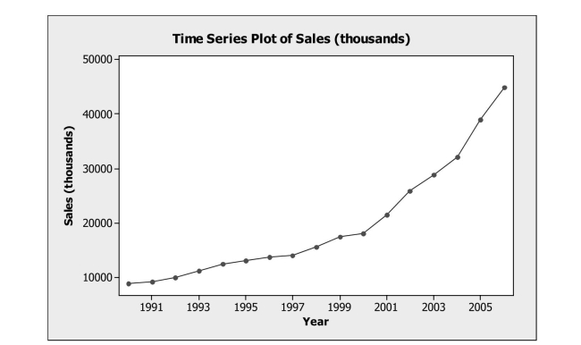
A) Moving Average
B) Single Exponential Smoothing
C) Quadratic Trend
D) Linear Trend
E) Seasonal Regression
For a well known department store chain. Which model would be most appropriate for
Forecasting this series?
A) Moving Average
B) Single Exponential Smoothing
C) Quadratic Trend
D) Linear Trend
E) Seasonal Regression
Question
Stock prices and earnings per share (EPS) data were collected for a sample of 15
Companies. A regression model was fit to these data. From its plots of residuals shown
Below, which assumption appears to be violated?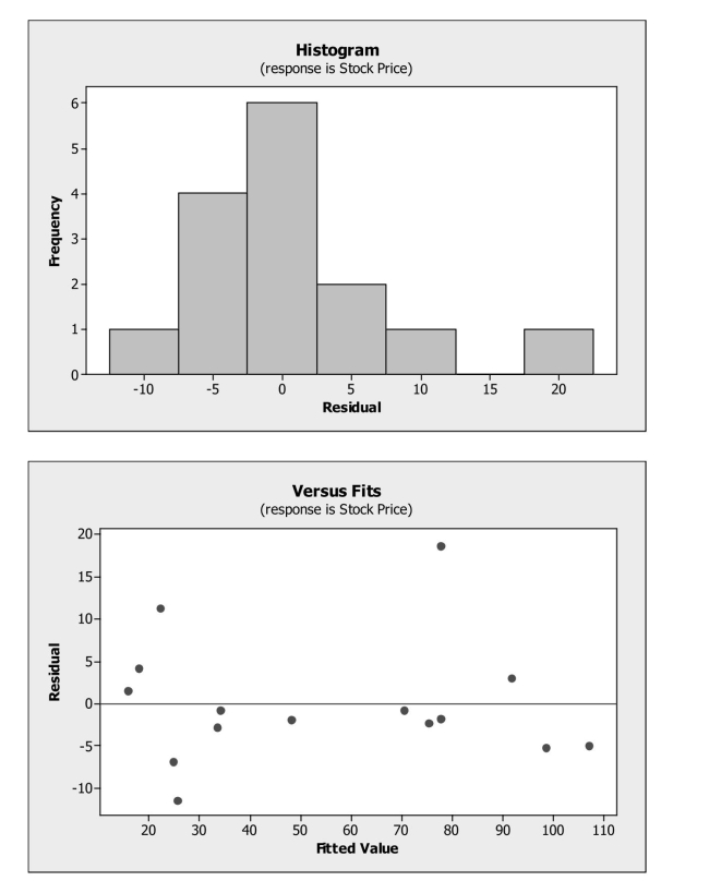
A) Equal Variance
B) Linearity
C) Normality
D) Independence
E) None; all appear to be satisfied.
Companies. A regression model was fit to these data. From its plots of residuals shown
Below, which assumption appears to be violated?
A) Equal Variance
B) Linearity
C) Normality
D) Independence
E) None; all appear to be satisfied.
Question
Question
Question
Question
A least squares estimated regression line has been fitted to a set of data and the
Resulting residual plot is shown. Which is true?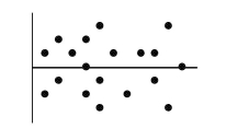
A) The linear model is appropriate.
B) The linear model is poor because some residuals are large.
C) The linear model is poor because the correlation is near 0.
D) A curved model would be better.
E) A transformation of the data is required.
Resulting residual plot is shown. Which is true?
A) The linear model is appropriate.
B) The linear model is poor because some residuals are large.
C) The linear model is poor because the correlation is near 0.
D) A curved model would be better.
E) A transformation of the data is required.
Question
Question
Question
Question
Question
If the point in the upper left corner of the scatterplot shown below is removed,
What will happen to the correlation (r) and the slope of the line of best fit (b)?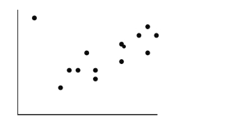
A) They will not change.
B) Both will increase.
C) Both will decrease.
D) r will increase and b will decrease.
E) r will decrease and b will increase.
What will happen to the correlation (r) and the slope of the line of best fit (b)?
A) They will not change.
B) Both will increase.
C) Both will decrease.
D) r will increase and b will decrease.
E) r will decrease and b will increase.
Question
Question
Question
Question
Question
Question
The time series graph below shows annual sales figures (in thousands of dollars)
For a well known department store chain. The dominant component in these data is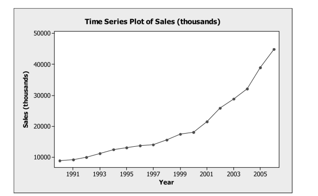
A) Trend
B) Seasonal
C) Randomness
D) Irregular
E) Error
For a well known department store chain. The dominant component in these data is
A) Trend
B) Seasonal
C) Randomness
D) Irregular
E) Error
Question
Question
Question
Question
Question
In order to examine if the size of cash bonuses depends on pay scale, data were
Obtained on the average annual cash bonus and the average annual pay for a sample of 20
Companies. A regression model was fit to these data. From its plot of residuals versus
Fitted values shown below, which assumption appears to be violated?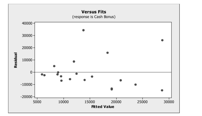
A) Equal Variance
B) Linearity
C) Normality
D) Independence
E) None; all appear to be satisfied.
Question
Question
Question
Question
The residual plot for a linear regression model is shown below. Which of the
Following statements is true?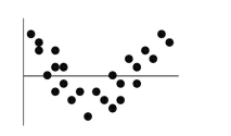
A) The linear model is okay because the same number of points is above the line as below it.
B) The linear model is okay because the association between the two variables is fairly strong.
C) The linear model is no good because the correlation is near 0.
D) The linear model is no good because some residuals are large.
E) The linear model is no good because of the curve in the residuals.
Question
Question
Weekly commodity prices for heating oil (in cents) were obtained and regressed
Against time. The residual plots from fitting the linear model are shown below. Which
Assumptions appear to be violated?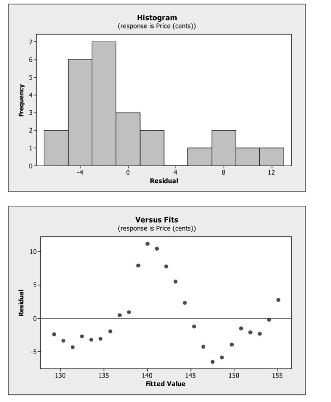
A) Linearity
B) Normality
C) Equal Variance
D) Both A and B
E) All of the above
Against time. The residual plots from fitting the linear model are shown below. Which
Assumptions appear to be violated?
A) Linearity
B) Normality
C) Equal Variance
D) Both A and B
E) All of the above
Question
The time series graph below shows monthly sales figures for a specialty gift item
Sold on the Home Shopping Network (HSN). The dominant component in these data is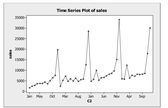
A) Cyclical
B) Seasonal
C) Randomness
D) Irregular
E) Error
Sold on the Home Shopping Network (HSN). The dominant component in these data is
A) Cyclical
B) Seasonal
C) Randomness
D) Irregular
E) Error
Question
Question
Question
Question
Question
Question
Question

Unlock Deck
Sign up to unlock the cards in this deck!
Unlock Deck
Unlock Deck
1/38
Play
Full screen (f)
Deck 29: Models for Decision Making
1
Quarterly returns were forecasted for a mutual fund comprised of technology
Stocks. The forecast errors for the last six quarters are as follows: -.47, 1.12, -.85, 1.27,
)07, and -.05. The MSE based on these forecast errors is
A) .77
B) .98
C) .22
D) .18
E) .64
Stocks. The forecast errors for the last six quarters are as follows: -.47, 1.12, -.85, 1.27,
)07, and -.05. The MSE based on these forecast errors is
A) .77
B) .98
C) .22
D) .18
E) .64
E
2
Which statement about re-expressing data is not true?
I) Unimodal distributions that are skewed to the left can be made more
Symmetric by taking the square root of the variable.
II) A curve that is descending as the explanatory variable increases may be
Straightened by taking a logarithm of the response variable.
III) One goal of re-expression may be to make the variability of the response
Variable more uniform.
A) I only
B) II only
C) III only
D) II and III
E) I, II and III
D
3
The time series graph below shows annual sales figures (in thousands of dollars)
For a well known department store chain. Which model would be most appropriate for
Forecasting this series?
A) Moving Average
B) Single Exponential Smoothing
C) Quadratic Trend
D) Linear Trend
E) Seasonal Regression
For a well known department store chain. Which model would be most appropriate for
Forecasting this series?
A) Moving Average
B) Single Exponential Smoothing
C) Quadratic Trend
D) Linear Trend
E) Seasonal Regression
C
4
Stock prices and earnings per share (EPS) data were collected for a sample of 15
Companies. A regression model was fit to these data. From its plots of residuals shown
Below, which assumption appears to be violated?
A) Equal Variance
B) Linearity
C) Normality
D) Independence
E) None; all appear to be satisfied.
Companies. A regression model was fit to these data. From its plots of residuals shown
Below, which assumption appears to be violated?
A) Equal Variance
B) Linearity
C) Normality
D) Independence
E) None; all appear to be satisfied.
Unlock Deck
Unlock for access to all 38 flashcards in this deck.
Unlock Deck
k this deck
5
Stock prices and earnings per share (EPS) data were collected for a sample of 15
Companies. Below are the regression results. Which of the following statement is true
About the correlation between stock price and EPS? The regression equation is
Stock Price EPS
A) The correlation is negative.
B) The correlation is not significantly different from zero.
C) The correlation is positive and significantly different from zero.
D) The correlation is positive but not significantly different from zero.
E) Cannot be determined from the information given.
Unlock Deck
Unlock for access to all 38 flashcards in this deck.
Unlock Deck
k this deck
6
The regression model developed to predict a firm's Price-Earnings Ratio (PE)
Based on Growth Rate, Profit Margin, and whether or not the firm is Green (1 = Yes, 0 =
no. is
Which of the following is the correct interpretation for the regression coefficient of
Green?
A) The regression coefficient indicates that the PE ratio of a firm that is green will, on average, be 2.09 higher than a firm that is not green with the same growth rate
And profit margin.
B) The regression coefficient indicates that the PE ratio of a firm that is green will, on average, be 2.09 lower than a firm that is not green with the same growth rate
And profit margin.
C) The regression coefficient indicates that the PE ratio of a firm that is green will, on average, be 2.09 times higher than a firm that is not green with the same
Growth rate and profit margin.
D) The regression coefficient indicates that the PE ratio of a firm that is green will, on average, be 2.09 times lower than a firm that is not green with the same
Growth rate and profit margin.
E) The regression coefficient is not significantly different from zero.
Unlock Deck
Unlock for access to all 38 flashcards in this deck.
Unlock Deck
k this deck
7
Data were collected for a sample of 12 pharmacists to determine if years of
Experience and salary are related. Below are the regression analysis results. The
Dependent variable is Salary in thousands of dollars. How much of the variability in
Pharmacists' salary is accounted for by years of experience? Regression Analysis: Salary versus Years Experience
The regression equation is
Salary Years Experience
A) 82.8 %
B) 47.97 %
C) 5.58485 thousands dollars
D) 10.99 %
E) 98.9 %
Unlock Deck
Unlock for access to all 38 flashcards in this deck.
Unlock Deck
k this deck
8
A least squares estimated regression line has been fitted to a set of data and the
Resulting residual plot is shown. Which is true?
A) The linear model is appropriate.
B) The linear model is poor because some residuals are large.
C) The linear model is poor because the correlation is near 0.
D) A curved model would be better.
E) A transformation of the data is required.
Resulting residual plot is shown. Which is true?
A) The linear model is appropriate.
B) The linear model is poor because some residuals are large.
C) The linear model is poor because the correlation is near 0.
D) A curved model would be better.
E) A transformation of the data is required.
Unlock Deck
Unlock for access to all 38 flashcards in this deck.
Unlock Deck
k this deck
9
Data were collected for a sample of 12 pharmacists to determine if years of
Experience and salary are related. The regression model fit to these data is
Using this regression equation to predict
Salary for 10 years of experience gives the following results. Which of the following is
True?
A) 95% of pharmacists with 10 years of experience earn between $38,960 and $65,130.
B) 95% of pharmacists with 10 years of experience earn between $48,010 and $56,080.
C) We are 95% confident that a particular pharmacist who has 10 years of experience earns between $38,960 and $65,130.
D) We are 95% confident that a particular pharmacist who has 10 years of experience earns between $48,010 and $56,080
E) 95% of pharmacists with 10 years experience on average earn between $48,010
Unlock Deck
Unlock for access to all 38 flashcards in this deck.
Unlock Deck
k this deck
10
Quarterly returns were forecasted for a mutual fund comprised of technology
Stocks. The forecast errors for the last six quarters are as follows: -.47, 1.12, -.85, 1.27,
)07, and -.05. The MAD based on these forecast errors is
A) .77
B) .98
C) .22
D) .18
E) .64
Stocks. The forecast errors for the last six quarters are as follows: -.47, 1.12, -.85, 1.27,
)07, and -.05. The MAD based on these forecast errors is
A) .77
B) .98
C) .22
D) .18
E) .64
Unlock Deck
Unlock for access to all 38 flashcards in this deck.
Unlock Deck
k this deck
11
A first-order autoregressive model, AR (1) was fit to monthly closing stock
Prices, adjusted for dividends, of Boeing Corporation from January 2006 through August
2008 (closing price on the first trading day of the month). Based on the results shown
Below, the forecast a month in which the previous month's closing price was $67.52 is
A) $74.06
B) $68.26
C) $65.67
D) $71.25
E) Cannot be determined from the information given.
Unlock Deck
Unlock for access to all 38 flashcards in this deck.
Unlock Deck
k this deck
12
Data were collected for a sample of 12 pharmacists to determine if years of
Experience and salary are related. Below are the regression analysis results. The
Dependent variable is Salary in thousands of dollars. The standard error of the slope for
This estimated regression equation is
Regression Analysis: Salary versus Years Experience The regression equation is
Salary Years Experience
A) 3.381
B) 0.2149
C) 5.58485
D) 82.8
E) 1.4882
Unlock Deck
Unlock for access to all 38 flashcards in this deck.
Unlock Deck
k this deck
13
If the point in the upper left corner of the scatterplot shown below is removed,
What will happen to the correlation (r) and the slope of the line of best fit (b)?
A) They will not change.
B) Both will increase.
C) Both will decrease.
D) r will increase and b will decrease.
E) r will decrease and b will increase.
What will happen to the correlation (r) and the slope of the line of best fit (b)?
A) They will not change.
B) Both will increase.
C) Both will decrease.
D) r will increase and b will decrease.
E) r will decrease and b will increase.
Unlock Deck
Unlock for access to all 38 flashcards in this deck.
Unlock Deck
k this deck
14
Data were collected for a sample of 12 pharmacists to determine if years of
Experience and salary are related. Below are the regression analysis results. The
Dependent variable is Salary in thousands of dollars. The calculated t-statistic to test
Whether the regression slope is significant is
Regression Analysis: Salary versus Years Experience The regression equation is
Salary Years Experience
A) 10.99
B) 47.97
C) 31.2
D) 6.93
E) 5.58485
Unlock Deck
Unlock for access to all 38 flashcards in this deck.
Unlock Deck
k this deck
15
Which of the following measures is used to check for collinearity when building a
Multiple regression model?
A) Cook's Distance
B) Variance Inflation Factor
C) Determination Coefficient
D) Standardized Residual
E) Chef's Distance
Multiple regression model?
A) Cook's Distance
B) Variance Inflation Factor
C) Determination Coefficient
D) Standardized Residual
E) Chef's Distance
Unlock Deck
Unlock for access to all 38 flashcards in this deck.
Unlock Deck
k this deck
16
A linear regression model was fit to data collected over a 13 year period
Representing technology adoption over time. Based on the regression output below, the
Durbin Watson statistic indicates
Regression Analysis: Technology Adoption versus Time The regression equation is
Technology Adoption Time
Durbin-Watson statistic
A) that the residuals are positively autocorrelated.
B) that the residuals are negatively autocorrelated.
C) that the residuals are not autocorrelated.
D) that the test is inconclusive.
E) none of the above; the Durbin Watson cannot be used for this model.
Unlock Deck
Unlock for access to all 38 flashcards in this deck.
Unlock Deck
k this deck
17
Stock prices and earnings per share (EPS) data were collected for a sample of 15
Companies. Below are the regression results. The dependent variable is Stock Price.
What is the correlation between stock price and EPS?
Regression Analysis: Stock Price versus EPS The regression equation is
Stock Price EPS
A) -.975
B) .975
C) .906
D) .950
E) Cannot be determined from the information given.
Unlock Deck
Unlock for access to all 38 flashcards in this deck.
Unlock Deck
k this deck
18
The following is output from regression analysis performed to develop a model
For predicting a firm's Price-Earnings Ratio (PE) based on Growth Rate, Profit Margin,
And whether or not the firm is Green (1 = Yes, 0 = No). At = .05 we can conclude that
? The regression equation is
Growth Rate Profit Margin Green?
A) Growth Rate is not a significant variable in predicting a firm's PE ratio.
B) Profit Margin is a significant variable in predicting a firm's PE ratio.
C) The regression coefficient associated with Growth Rate is not significantly different from zero.
D) Whether or not a firm is Green is significant in predicting its PE ratio.
E) The regression coefficient associated with Profit Margin is significantly different
Unlock Deck
Unlock for access to all 38 flashcards in this deck.
Unlock Deck
k this deck
19
The time series graph below shows annual sales figures (in thousands of dollars)
For a well known department store chain. The dominant component in these data is
A) Trend
B) Seasonal
C) Randomness
D) Irregular
E) Error
For a well known department store chain. The dominant component in these data is
A) Trend
B) Seasonal
C) Randomness
D) Irregular
E) Error
Unlock Deck
Unlock for access to all 38 flashcards in this deck.
Unlock Deck
k this deck
20
The model predicted can be used to predict the
Stopping distance (in feet) for a car traveling at a specific speed (in mph). According to
This model, about how much distance will a car going 65 mph need to stop?
A) 345.0 feet
B) 18.6 feet
C) 27.0 feet
D) 4.3 feet
E) 729.0 feet
Stopping distance (in feet) for a car traveling at a specific speed (in mph). According to
This model, about how much distance will a car going 65 mph need to stop?
A) 345.0 feet
B) 18.6 feet
C) 27.0 feet
D) 4.3 feet
E) 729.0 feet
Unlock Deck
Unlock for access to all 38 flashcards in this deck.
Unlock Deck
k this deck
21
Based on the actual and forecasted returns for a social choice portfolio shown
Below, the MAD is
A) 0.507
B) 2.344
C) 0.249
D) 1.531
E) None of the above
Below, the MAD is
A) 0.507
B) 2.344
C) 0.249
D) 1.531
E) None of the above
Unlock Deck
Unlock for access to all 38 flashcards in this deck.
Unlock Deck
k this deck
22
Which statement about influential points is true?
I) Removal of an influential point changes the regression line.
II) A high leverage point is always influential.
III) Influential points have large residuals.
A) I only
B) I and II
C) I and III
D) II and III
E) I, II and III
I) Removal of an influential point changes the regression line.
II) A high leverage point is always influential.
III) Influential points have large residuals.
A) I only
B) I and II
C) I and III
D) II and III
E) I, II and III
Unlock Deck
Unlock for access to all 38 flashcards in this deck.
Unlock Deck
k this deck
23
In order to examine if there is a relationship between the size of cash bonuses and
Pay scale, data were obtained on the average annual cash bonus and the average annual
Pay for a sample of 20 companies. Below is the regression analysis output with annual
Cash bonus as the dependent variable. What is the correlation between average annual
Cash bonus and average annual pay?
Regression Analysis: Cash Bonus versus Pay The regression equation is
Cash Bonus Pay
A) -.223
B) .472
C) .108
D) -.540
E) Cannot be determined from the information given.
Unlock Deck
Unlock for access to all 38 flashcards in this deck.
Unlock Deck
k this deck
24
In order to examine if the size of cash bonuses depends on pay scale, data were
Obtained on the average annual cash bonus and the average annual pay for a sample of 20
Companies. A regression model was fit to these data. From its plot of residuals versus
Fitted values shown below, which assumption appears to be violated?
A) Equal Variance
B) Linearity
C) Normality
D) Independence
E) None; all appear to be satisfied.
Obtained on the average annual cash bonus and the average annual pay for a sample of 20
Companies. A regression model was fit to these data. From its plot of residuals versus
Fitted values shown below, which assumption appears to be violated?
A) Equal Variance
B) Linearity
C) Normality
D) Independence
E) None; all appear to be satisfied.
Unlock Deck
Unlock for access to all 38 flashcards in this deck.
Unlock Deck
k this deck
25
A large pharmaceutical company selected a random sample of new hires and
Obtained their job performance ratings based on their first six months with the company.
These data were used to build a multiple regression model to predict the job performance
Of new hires based on age, GPA and gender (female = 1 and male = 0). The results of
The analysis are shown below. How much of the variability in Job Performance is
Explained by the regression model? The regression equation is
Job Performance Age GPA Gender
A) 30.33 %
B) 77.7 %
C) 5.56 %
D) 60.76 %
E) cannot be determined.
Unlock Deck
Unlock for access to all 38 flashcards in this deck.
Unlock Deck
k this deck
26
A farmer has increased his wheat production by about the same amount each year.
His most useful predictive model is most probably
A) exponential.
B) linear.
C) logarithmic.
D) power.
E) quadratic.
His most useful predictive model is most probably
A) exponential.
B) linear.
C) logarithmic.
D) power.
E) quadratic.
Unlock Deck
Unlock for access to all 38 flashcards in this deck.
Unlock Deck
k this deck
27
A large pharmaceutical company selected a random sample of new hires and
Obtained their job performance ratings based on their first six months with the company.
These data were used to build a multiple regression model to predict the job performance
Of new hires based on age, GPA and gender (female = 1 and male = 0). The regression
Equation is:
Which of the following is the correct interpretation for the regression coefficient of
Gender?
A) The regression coefficient indicates that the job performance score for a female will, on average, be 9.06 points higher than for males of the same age and GPA.
B) The regression coefficient indicates that the job performance score for a female will, on average, be 9.06 points lower than for males of the same age and GPA.
C) The regression coefficient indicates that the job performance score for a female will, on average, be 9.06 times higher than for males.
D) The regression coefficient indicates that the job performance score for a female will, on average, be 9.06 times lower than for males.
E) The regression coefficient is not significantly different from zero.
Unlock Deck
Unlock for access to all 38 flashcards in this deck.
Unlock Deck
k this deck
28
The residual plot for a linear regression model is shown below. Which of the
Following statements is true?
A) The linear model is okay because the same number of points is above the line as below it.
B) The linear model is okay because the association between the two variables is fairly strong.
C) The linear model is no good because the correlation is near 0.
D) The linear model is no good because some residuals are large.
E) The linear model is no good because of the curve in the residuals.
Following statements is true?
A) The linear model is okay because the same number of points is above the line as below it.
B) The linear model is okay because the association between the two variables is fairly strong.
C) The linear model is no good because the correlation is near 0.
D) The linear model is no good because some residuals are large.
E) The linear model is no good because of the curve in the residuals.
Unlock Deck
Unlock for access to all 38 flashcards in this deck.
Unlock Deck
k this deck
29
A large pharmaceutical company selected a random sample of new hires and
Obtained their job performance ratings based on their first six months with the company.
These data were used to build a multiple regression model to predict the job performance
Of new hires based on age, GPA and gender (female = 1 and male = 0). The results of
The analysis are shown below. At = .05 we can conclude that
? The regression equation is
Job Performance Age Gender
A) Age is not a significant variable in predicting job performance.
B) GPA is a significant variable in predicting job performance.
C) The regression coefficient associated with GPA is significantly different from zero.
D) Gender is a significant variable in predicting job performance.
E) The regression coefficient associated with Age is not significantly different from
Unlock Deck
Unlock for access to all 38 flashcards in this deck.
Unlock Deck
k this deck
30
Weekly commodity prices for heating oil (in cents) were obtained and regressed
Against time. The residual plots from fitting the linear model are shown below. Which
Assumptions appear to be violated?
A) Linearity
B) Normality
C) Equal Variance
D) Both A and B
E) All of the above
Against time. The residual plots from fitting the linear model are shown below. Which
Assumptions appear to be violated?
A) Linearity
B) Normality
C) Equal Variance
D) Both A and B
E) All of the above
Unlock Deck
Unlock for access to all 38 flashcards in this deck.
Unlock Deck
k this deck
31
The time series graph below shows monthly sales figures for a specialty gift item
Sold on the Home Shopping Network (HSN). The dominant component in these data is
A) Cyclical
B) Seasonal
C) Randomness
D) Irregular
E) Error
Sold on the Home Shopping Network (HSN). The dominant component in these data is
A) Cyclical
B) Seasonal
C) Randomness
D) Irregular
E) Error
Unlock Deck
Unlock for access to all 38 flashcards in this deck.
Unlock Deck
k this deck
32
Based on returns for the last six months of 2007 for a social choice portfolio
Comprised of "green" companies shown below, the forecasted monthly return for January
2008 using a three-month moving average is
A) 1.77
B) 1.9
C) 1.55
D) 2.47
E) 1.47
Comprised of "green" companies shown below, the forecasted monthly return for January
2008 using a three-month moving average is
A) 1.77
B) 1.9
C) 1.55
D) 2.47
E) 1.47
Unlock Deck
Unlock for access to all 38 flashcards in this deck.
Unlock Deck
k this deck
33
Weekly commodity prices for heating oil (in cents) were obtained for a period of
30 weeks and regressed against time. Based on the regression output shown below, the
Durbin-Watson statistic indicates The regression equation is
Price (cents) Time
Durbin-Watson statistic
A) that the residuals are positively autocorrelated.
B) that the residuals are negatively autocorrelated.
C) that the residuals are not autocorrelated.
D) that the test is inconclusive.
E) none of the above; the Durbin Watson cannot be used for this model.
Unlock Deck
Unlock for access to all 38 flashcards in this deck.
Unlock Deck
k this deck
34
For many countries tourism is an important source of revenue. Data are collected
On the number of foreign visitors to a country (in millions) and total tourism revenue (in
Billions of dollars) for a sample of 10 countries. Below is the regression analysis output
With tourism revenue as the dependent variable. The standard error of the slope for this
Estimated regression equation is Regression Analysis: Tourism (\$ bill) versus Visitors (mill)
The regression equation is
Tourism bill visitors
A) 2.58307
B) 3.462
C) 0.07917
D) 6.672
E) 0.29497
Unlock Deck
Unlock for access to all 38 flashcards in this deck.
Unlock Deck
k this deck
35
For many countries tourism is an important source of revenue. Data are collected
On the number of foreign visitors to a country (in millions) and total tourism revenue (in
Billions of dollars) for a sample of 10 countries. Below is partial regression analysis
Output with tourism revenue as the dependent variable. How much of the variability in
Tourism revenue is accounted for by the number of foreign visitors?
Regression Analysis: Tourism ($ bill) versus Visitors (mill) The regression equation is
Tourism bill Visitors (mill)
A) 63.4 %
B) 13.8 %
C) 2.58 billion $
D) 21.464 %
E) 3.73 billion $
Unlock Deck
Unlock for access to all 38 flashcards in this deck.
Unlock Deck
k this deck
36
In order to examine if there is a relationship between the size of cash bonuses and
Pay scale, data were obtained on the average annual cash bonus and the average annual
Pay for a sample of 20 companies. Below is the regression analysis output with annual
Cash bonus as the dependent variable. Which of the following statement is true about the
Correlation between average annual cash bonus and average annual pay using
? = 0.05?
Regression Analysis: Cash Bonus versus Pay The regression equation is
Cash Bonus Pay
A) It is not significantly different from zero.
B) It is negative but not significantly different from zero.
C) It is positive and significantly different from zero.
D) It is negative and significantly different from zero.
E) Cannot be determined from the information given.
Unlock Deck
Unlock for access to all 38 flashcards in this deck.
Unlock Deck
k this deck
37
For many countries tourism is an important source of revenue. Data are collected
On the number of foreign visitors to a country (in millions) and total tourism revenue (in
Billions of dollars) for a sample of 10 countries. Below is partial regression analysis
Output with tourism revenue as the dependent variable. The calculated t-statistic to test
Whether the regression slope is significant is
Regression Analysis: Tourism ($ bill) versus Visitors (mill) The regression equation is
Tourism bill Visitors (mill)
A) 6.20
B) 13.88
C) 0.07917
D) 2.58307
E) 3.73
Unlock Deck
Unlock for access to all 38 flashcards in this deck.
Unlock Deck
k this deck
38
For many countries tourism is an important source of revenue. Data are collected
On the number of foreign visitors to a country (in millions) and total tourism revenue (in
Billions of dollars) for a sample of 10 countries. The regression equation fit was
If we were interested in
Predicting the tourism revenue for a particular country that had 30 million foreign
Visitors,
A) we should construct a confidence interval using this equation.
B) we should construct a predication interval using this equation.
C) we should not use this equation because it is not significant.
D) we should use the correlation.
E) we should use the standard error.
Unlock Deck
Unlock for access to all 38 flashcards in this deck.
Unlock Deck
k this deck
Unlock Deck
Unlock for access to all 38 flashcards in this deck.


