Deck 3: Univariate Population Parameters and Sample Statistics

Question 1

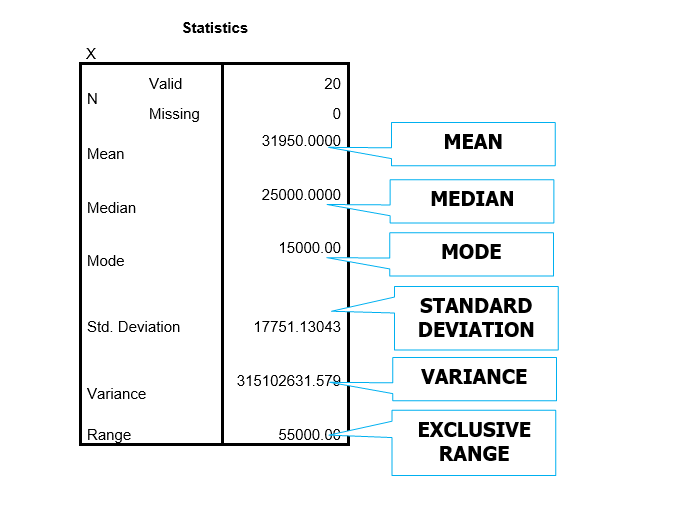
For the following data, and assuming an interval width of 1, compute the following:

$\begin{array}{r}\hline X \\\hline 25 \\21 \\16 \\18 \\19 \\21 \\21 \\22 \\17 \\19 \\\hline\end{array}$

a. Mode
b. Median
c. Mean
d. Exclusive and inclusive range
e. H spread
f. Variance and standard deviation

Answer 1

a. Mode.
This is the most frequently occurring value in the dataset.

Based on the frequency distribution, we see the mode is 21 as it has a frequency of 3.

$\begin{array}{|r|r|r|r|r|} \hline&& ×\\& \text { Frequency } &{\text { Percent }} & \text { Valid Percent } &{\text { Cumulative }} \\&&&&\text { Percent }\\\hline 16.00 & 1 & 10.0 & 10.0 & 10.0 \\17.00 & 1 & 10.0 & 10.0 & 20.0 \\18.00 & 1 & 10.0 & 10.0 & 30.0 \\19.00 & 2 & 20.0 & 20.0 & 50.0 \\\text { Valid }21.00 & 3 & 30.0 & 30.0 & 80.0 \\22.00 & 1 & 10.0 & 10.0 & 90.0 \\25.00 & 1 & 10.0 & 10.0 & 100.0\\ \text { Total } & 10 & 100.0 & 100.0 \\\hline\end{array}$

b. Median.
$\text { Median }=L R L+\frac{50 \%(n)-c f}{f} w=18.5+\frac{50 \%(10)-3}{2}(1)=18.5+\frac{2}{2}(1)=18.5$ LRL is the lower real limit of the interval containing the median (in this case, 18.5 as the median is contained in the interval with the value of 19) , 50% is the percentile desired, n is the sample size (in this case 10), cf is the cumulative frequency of all intervals less than but not including the interval containing the median (cf below; in this case we can look at the frequency distribution and see that the cf = 1 + 1 + 1 = 3), f is the frequency of the interval containing the median (which in this case is 2), and w is the interval width (which in this case is 1).

Generating the median using SPSS we find:

c. Mean.
The sum of all the Xs is 2300 and the sample size is 50. Thus the mean is 46 (as seen here).
$\bar{X}=\frac{\sum_{i=1}^{n} X_{i}}{n}=\frac{199}{10}=19.90$
Generating the mean using SPSS we find:


d. Exclusive and inclusive range.
The exclusive range is defined as the difference between the largest and smallest scores in a collection of scores. For notational purposes, the exclusive range (ER) is shown as ER = X??? - X???. As seen previously in the frequency distribution, the largest and smallest values, respectively, are 25 and 16.
Thus ER = 25 - 16 = 9.
The inclusive range takes into account the interval width so that all scores are included in the range. The inclusive range is defined as the difference between the upper real limit of the interval containing the largest score and the lower real limit of the interval containing the smallest score in a collection of scores. For notational purposes, the inclusive range (IR) is shown as IR = URL of X- LRL of X. For this example, with an interval width of one, IR = 25.5 - 15.5 = 10.

e. H spread.
H spread is defined as Q?- Q?, the simple difference between the third and first quartiles. Using SPSS and computing the quartiles with values at group midpoints, we find the first and third quartiles as follows and the resulting H spread: H = Q1- Q2= 21.25 - 17.75 = 3.50. [Had this been computed not using values at group midpoints, H = Q1- Q2 = 21.500 - 18.000 = 3.500.]


f. Variance and standard deviation.
The sample variance is computed as:
$s^{2}=\frac{n \sum_{i=1}^{n} X_{i}^{2}-\left(\sum_{i=1}^{n} X_{i}\right)^{2}}{n(n-1)}$
Based on this formula, we need to compute X², the sum of X², and the sum of X:

$\begin{array}{l}\begin{array}{rr}\hline X & X^{2} \\\hline 25 & 625 \\21 & 441 \\16 & 256 \\18 & 324 \\19 & 361 \\21 & 441 \\21 & 441 \\22 & 484 \\17 & 289 \\19 & 361 \\\hline\\199&4023 &\text { SUM }\end{array}\\\end{array}$

Plugging the values into the formula, we find the variance:
$s^{2}=\frac{n \sum_{i=1}^{n} X_{i}^{2}-\left(\sum_{i=1}^{n} X_{i}\right)^{2}}{n(n-1)}=\frac{10(4023)-(199)^{2}}{10(10-1)}=\frac{40230-39601}{90}=6.98889$ And the standard deviation is:
$s=+\sqrt{s^{2}}=\sqrt{6.98889}=2.64365$
Computed the variance and standard deviation using SPSS, we find:

Question 2

For the following data, and assuming an interval width of 1, compute the following using SPSS:
a. Mode
b. Median
c. Mean
d. Exclusive range
e. Standard deviation
f. Variance

$\begin{array}{r}\hline X \\\hline15000 \\15000 \\15000 \\15000 \\15000 \\15000 \\15000 \\25000 \\25000 \\25000 \\25000 \\25000 \\42000 \\42000 \\45000 \\45000 \\50000 \\50000 \\65000 \\70000 \\\hline\end{array}$

Answer 2

Question 3

Without doing any computations, which of the following distributions has the largest variance?

$\begin{array}{cccccc}\hline X & f & Y & f & Z & f \\\hline 64 & 1 & 50 & 2 & 80 & 3 \\66 & 1 & 60 & 2 & 81 & 2 \\69 & 5 & 75 & 2 & 82 & 2 \\74 & 2 & 80 & 2 & 83 & 2 \\76 & 1 & 85 & 6 & 84 & 2 \\78 & 4 & 90 & 2 & 85 & 4 \\79 & 1 & 95 & 2 & 86 & 2 \\80 & 5 & 100 & 2 & 87 & 3 \\\hline\end{array}$

Answer 3

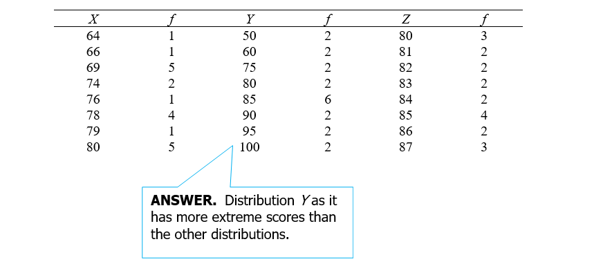
Question 4

Without doing any computations, which of the following distributions has the largest variance?

$\begin{array}{cccccc}\hline X & f & Y & f & Z & f \\\hline 30 & 3 & 41 & 2 & 45 & 3 \\36 & 2 & 42 & 4 & 46 & 1 \\40 & 3 & 44 & 2 & 48 & 1 \\41 & 2 & 45 & 4 & 51 & 3 \\48 & 2 & 51 & 2 & 53 & 3 \\50 & 3 & 52 & 2 & 55 & 3 \\52 & 2 & 53 & 2 & 59 & 3 \\60 & 3 & 54 & 2 & 60 & 3 \\\hline\end{array}$

Question 5

Without doing any computations, which of the following distributions has the largest variance?

$\begin{array}{cccccc}\hline X & f & Y & f & Z & f \\\hline 100 & 1 & 110 & 5 & 99 & 1 \\111 & 4 & 112 & 1 & 120 & 4 \\115 & 1 & 114 & 2 & 125 & 4 \\120 & 1 & 117 & 2 & 127 & 4 \\122 & 4 & 118 & 2 & 130 & 2 \\125 & 1 & 125 & 1 & 132 & 3 \\130 & 1 & 128 & 1 & 135 & 1 \\135 & 7 & 129 & 6 & 175 & 1 \\\hline\end{array}$

Question 6

The mean is a function of which scores in the distribution?

A) All but the two most extreme values
B) All but the one more extreme score
C) Every score
D) Only the largest and smallest scores
E) Only the middle two values
F) The most frequently occurring values

Question 7

For which measurement scales is computing the mean appropriate? Select all that apply.

A) Nominal
B) Ordinal
C) Interval
D) Ratio

Question 8

Compute the mean for the following values: 4, 8, 6, 1, 0, 9

A) 3.89
B) 4.67
C) 5.21
D) 6.00