Deck 17: Simple Linear Regression
Full screen (f)
Question
Question
Question
Question
Question
In which of the following situations is it most appropriate to use the simple linear regression model?
A)
B)
C)
D)
A)
B)
C)
D)
Question
Question
Question

Unlock Deck
Sign up to unlock the cards in this deck!
Unlock Deck
Unlock Deck
1/8
Play
Full screen (f)
Deck 17: Simple Linear Regression
1
You are given the following pairs of scores on X (Pretest score) and Y (Posttest score).
a. Find the linear regression model for predicting Y from X.
b. Use the prediction model obtained to predict the value of Y for a new person who scored 80 on the pretest.
a. Find the linear regression model for predicting Y from X.
b. Use the prediction model obtained to predict the value of Y for a new person who scored 80 on the pretest.
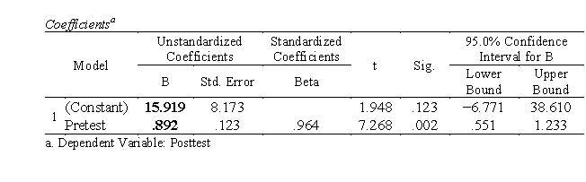
a. Intercept a = 15.919, slope b = .892.
The regression model is Yi = .892Xi + 15.919 + ei
The prediction equation is Yi = .892Xi + 15.919
b. When X = 80, Y' = .892X + 15.919 = .892(80) + 15.919 = 87.279Y'
Procedure:
Create a data set with two variables: Pretest (X), Posttest (Y). The data set should have 6 cases.
1) Go to Analyze Regression Linear.
2) Select Posttest to the Dependent list. Select Pretest to the Independent(s) list.
3) Click Statistics. Select Confidence interval under Regression Coefficients. Click Continue.
"4) Click OK.
Selected SPSS Output:
2
You are given the following pairs of scores on X (Percentage of students whose families are below poverty line) and Y (Percentage of students at or above proficiency level) for nine schools.
a. Find the linear regression model for predicting Y from X.
b. Use the prediction model obtained to predict the value of Y for a school that has 50% of students whose families are below the poverty line.
a. Find the linear regression model for predicting Y from X.
b. Use the prediction model obtained to predict the value of Y for a school that has 50% of students whose families are below the poverty line.
a. Intercept a = 15.919, slope b = .892.
The regression model is Yi = .892Xi + 15.919 + ei
The prediction equation is Y'i = .892Xi + 15.919
b. When X = 80, Y' = .892X + 15.919 = .892(80) + 15.919 = 87.279
Procedure:
Create a data set with two variables: Pretest (X), Posttest (Y). The data set should have 6 cases.
1. Go to Analyze Regression Linear.
2. Select Posttest to the Dependent list. Select Pretest to the Independent(s) list.
3. Click Statistics. Select Confidence interval under Regression Coefficients. Click Continue.
"4. Click OK.
Selected SPSS Output:
3
You are given the following pairs of scores on X (height in inches) and Y (weight in lbs).
Perform the following computations using = .05.
a. The regression equation of Y predicted by X.
b. Test of the significance of X as a predictor.
c. Plot Y versus X.
d. Compute the residuals.
e. Plot residuals versus X.
Perform the following computations using = .05.
a. The regression equation of Y predicted by X.
b. Test of the significance of X as a predictor.
c. Plot Y versus X.
d. Compute the residuals.
e. Plot residuals versus X.
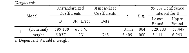
a. Intercept a = -199.139, slope b = 5.037.
The prediction equation is Y'i = 5.037Xi -199.139
b. Height is a good predictor of weight, F(1,23) = 29.262, p < .001. Additionally, the unstandardized slope (5.037) and standardized slope (.748) are statistically significantly different from 0 (t = 5.409, df = 23, p < .001); with every one inch increase in height, weight is expected to increase by 5.037 lbs.
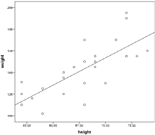
c. Plot of Y versus X.
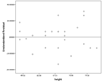
 (d) Residuals ei = Yi-Y'i.
(e) Plot of residuals versus X.
Procedure:
Create a data set with two variables: Height (X), Weight (Y). The data set should have 25 cases.
1) Go to Analyze Regression Linear.
2) Select Weight to the Dependent list. Select Height to the Independent(s) list.
3) Click Statistics. Select Confidence interval under Regression Coefficients. Click Continue.
4) To save residuals for the residual plot, click Save. Select Unstandardized under Residuals. Click Continue. Click OK.
5) To plot Y versus X, go to Graphs Legacy Dialogs Scatter/Dot. Select Simple Scatter. Click Define. Select Weight to Y axis, and Height to X axis. Click OK.
"6) To obtain the residual plot, go to Graphs Legacy Dialogs Scatter/Dot. Select Simple Scatter. Click Define. Select RES_1 to Y axis, and Height to X axis. Click OK.
Selected SPSS Output:
a. Predictors: (Constant), height
b. Dependent Variable: weight
The prediction equation is Y'i = 5.037Xi -199.139
b. Height is a good predictor of weight, F(1,23) = 29.262, p < .001. Additionally, the unstandardized slope (5.037) and standardized slope (.748) are statistically significantly different from 0 (t = 5.409, df = 23, p < .001); with every one inch increase in height, weight is expected to increase by 5.037 lbs.
c. Plot of Y versus X.
(d) Residuals ei = Yi-Y'i.(e) Plot of residuals versus X.
Procedure:
Create a data set with two variables: Height (X), Weight (Y). The data set should have 25 cases.
1) Go to Analyze Regression Linear.
2) Select Weight to the Dependent list. Select Height to the Independent(s) list.
3) Click Statistics. Select Confidence interval under Regression Coefficients. Click Continue.
4) To save residuals for the residual plot, click Save. Select Unstandardized under Residuals. Click Continue. Click OK.
5) To plot Y versus X, go to Graphs Legacy Dialogs Scatter/Dot. Select Simple Scatter. Click Define. Select Weight to Y axis, and Height to X axis. Click OK.
"6) To obtain the residual plot, go to Graphs Legacy Dialogs Scatter/Dot. Select Simple Scatter. Click Define. Select RES_1 to Y axis, and Height to X axis. Click OK.
Selected SPSS Output:
a. Predictors: (Constant), height
b. Dependent Variable: weight
4
Complete this sentence by selecting one of the following statements: "In simple linear regression, if the slope is found to be ?0.002, . . ."
A) the value of Y is equal to ?.002 when X is 0.
B) the value of Y is equal to ?.002 when X is 1.
C) the value of Y will decrease by 0.002 units when X increases by 1 unit.
D) there is a negative, but very weak relationship between X and Y.
A) the value of Y is equal to ?.002 when X is 0.
B) the value of Y is equal to ?.002 when X is 1.
C) the value of Y will decrease by 0.002 units when X increases by 1 unit.
D) there is a negative, but very weak relationship between X and Y.
Unlock Deck
Unlock for access to all 8 flashcards in this deck.
Unlock Deck
k this deck
5
In which of the following situations is it most appropriate to use the simple linear regression model?
A)
B)
C)
D)
A)
B)
C)
D)
Unlock Deck
Unlock for access to all 8 flashcards in this deck.
Unlock Deck
k this deck
6
Which one of the following reflects variables appropriate for a simple linear regression model?
A) One categorical dependent variable and one continuous independent variable
B) One continuous dependent variable and one continuous or categorical independent variable
C) One continuous dependent variable and two or more continuous independent variables
D) Two or more continuous dependent variables and one continuous or categorical independent variable
Unlock Deck
Unlock for access to all 8 flashcards in this deck.
Unlock Deck
k this deck
7
Which of the following is that part of the dependent variable that is not predicted by the independent variable?
A) Covariate
B) Intercept
C) Residual
D) Slope
A) Covariate
B) Intercept
C) Residual
D) Slope
Unlock Deck
Unlock for access to all 8 flashcards in this deck.
Unlock Deck
k this deck
8
The sample intercept is which of the following? Select all that apply.
A) The point where the regression line crosses the Y axis
B) The predicted change in Y for a one-unit change in X
C) The unstandardized regression coefficient
D) The value of the dependent variable when the independent variable is zero
A) The point where the regression line crosses the Y axis
B) The predicted change in Y for a one-unit change in X
C) The unstandardized regression coefficient
D) The value of the dependent variable when the independent variable is zero
Unlock Deck
Unlock for access to all 8 flashcards in this deck.
Unlock Deck
k this deck
Unlock Deck
Unlock for access to all 8 flashcards in this deck.


