Deck 6: Regression Analysis
Full screen (f)
Question
This represents which relationship?
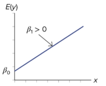
A) Positive linear
B) Negative linear
C) No linear
D) Multiple linear
A) Positive linear
B) Negative linear
C) No linear
D) Multiple linear
Question
Question
Question
Question
Question
Question
Question
Question
Question
Question
Question
Question
Question
Question
Question
Question
Question
Question
Based on the following table, what is the sample regression equation? 
A) Earnings = 10,625.6413 + 0.3731Cost + 174.0756Grad + 127.3845Debt
B) Earnings = 10,625.6413 + 0.373Cost + 174.0756Grad ? 127.385Debt
C) Earnings = 10,625.6413 ? 0.373Cost + 174.0756Grad ? 127.385Debt
D) Earnings = 10,625.6413 ? 0.373Cost + 174.0756Grad + 127.385 Debt
A) Earnings = 10,625.6413 + 0.3731Cost + 174.0756Grad + 127.3845Debt
B) Earnings = 10,625.6413 + 0.373Cost + 174.0756Grad ? 127.385Debt
C) Earnings = 10,625.6413 ? 0.373Cost + 174.0756Grad ? 127.385Debt
D) Earnings = 10,625.6413 ? 0.373Cost + 174.0756Grad + 127.385 Debt
Question
Based on the following table, what is the sample regression equation? 
A) Earnings = 10,004.9665 + 0.4349Cost + 178.0989Grad + 141.4783Debt
B) Earnings = 10,004.9665 ? 0.4349Cost + 178.0989Grad + 141.4783Debt
C) Earnings = 10,004.9665 + 0.4349Cost + 178.0989Grad ? 141.4783Debt
D) Earnings = 10,004.9665 ? 0.4349Cost + 178.0989Grad ? 141.4783 Debt
A) Earnings = 10,004.9665 + 0.4349Cost + 178.0989Grad + 141.4783Debt
B) Earnings = 10,004.9665 ? 0.4349Cost + 178.0989Grad + 141.4783Debt
C) Earnings = 10,004.9665 + 0.4349Cost + 178.0989Grad ? 141.4783Debt
D) Earnings = 10,004.9665 ? 0.4349Cost + 178.0989Grad ? 141.4783 Debt
Question
If there is a 30,000 average Service Cost in marketing services, with a 70% Cost Increase and 60% of client Payment for services upfront in addition to advantages of City, the predicted annual earnings for the firm are: 
A) $44,665.71
B) $37,890.63
C) $36,722.90
D) $47,392.23
A) $44,665.71
B) $37,890.63
C) $36,722.90
D) $47,392.23
Question
If there is a 30,000 average Service Cost in marketing services, with a 70% Cost Increase and 60% of client Payment for services upfront in addition to advantages of City, the predicted annual earnings for the firm are: 
A) $44,007.59
B) $35,518.89
C) $34,351.16
D) $46,534.38
A) $44,007.59
B) $35,518.89
C) $34,351.16
D) $46,534.38
Question
Question
Question
Question
The standard error of the estimate is Se = 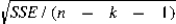 . What result best fits the sample data?< / p>
A) when Se = 1.526
B) when Se = 2.001
C) when Se = 0.543
D) when Se = 0.005
. What result best fits the sample data?< / p>A) when Se = 1.526
B) when Se = 2.001
C) when Se = 0.543
D) when Se = 0.005
Question
Based on goodness-of-fit measures, which is the preferred model based on the results below: 
A) model 1
B) model 2
C) model 3
D) Both model 1 & model 2
A) model 1
B) model 2
C) model 3
D) Both model 1 & model 2
Question
In the goodness-of-fit measures, interpret the coefficient of determination for Earnings with Model 3 and what the sample variation of earnings explains. 
A) 93.3700% of the sample variation in Earnings is explained by the regression model.
B) 0.8475 of the sample variation in Earnings determines the model selection.
C) 0.01 of the sample variation in Earnings determines the model selection.
D) 71.77% of the sample variation in Earnings is explained by the regression model.
Question
In the goodness-of-fit measures, interpret the coefficient of determination for Earnings with Model 3 and what the sample variation of earnings explains. 
A) 41.87% of the sample variation in Earnings is explained by the regression model.
B) 0.8475 of the sample variation in Earnings determines the model selection.
C) 0.010 of the sample variation in Earnings determines the model selection.
D) 42.88% of the sample variation in Earnings is explained by the regression model.
Question
Based on goodness-of-fit measures, what is the percentage of the sample variation unexplained by Model 2? 
A) 81.74%
B) 2.56%
C) 83.61%
D) 18.26%
A) 81.74%
B) 2.56%
C) 83.61%
D) 18.26%
Question
Based on goodness-of-fit measures, what is the percentage of the sample variation unexplained by Model 2? 
A) 38.90%
B) 40.23%
C) 41.87%
D) 59.77%
A) 38.90%
B) 40.23%
C) 41.87%
D) 59.77%
Question
Conduct a test to determine if the predictor variables are jointly significant in explaining Earnings at = 0.05. 
A) P(F1,18) 74.608, p-value is less than = 0.05, we reject H0, but jointly significant in explaining earnings.
B) P(F1,19) 82.818, p-value is less than = 0.05, we accept H0, jointly do not explain earnings.
C) P(F1,18) 74.608, p-value is less than = 0.05, we accept H0, but jointly significant in explaining earnings.
D) P(F1,19) 82.818, p-value is less than = 0.05, we reject H0, jointly do not explain earnings.
Question
Conduct a test to determine if the predictor variables are jointly significant in explaining Earnings at = 0.05. 
A) P(F1,18) 57.737, p-value is less than = 0.05, we reject H0, but jointly significant in explaining earnings.
B) P(F1,19) 60.945, p-value is less than = 0.05, we accept H0, but jointly significant in explain earnings.
C) P(F1,18) 57.737, p-value is less than = 0.05, we accept H0, but jointly significant in explaining earnings.
D) P(F1,19) 60.945, p-value is less than = 0.05, we reject H0, jointly do not explain earnings.
Question
Question
Question
Question
Question
Question
Question
Question
Question
Question
Question
Question
Question
Question
Question
Question
Question
Question
Question
Question

Unlock Deck
Sign up to unlock the cards in this deck!
Unlock Deck
Unlock Deck
1/53
Play
Full screen (f)
Deck 6: Regression Analysis
1
This represents which relationship?
A) Positive linear
B) Negative linear
C) No linear
D) Multiple linear
A) Positive linear
B) Negative linear
C) No linear
D) Multiple linear
Positive linear
2
The Department of Natural Resources conducted a study examining the condition of fish in the Wolfe River (Wisconsin). In total 110 fish were captured. The variables that were measured are: mile marker of location in river, species (rainbow trout, northern pike, musky, walleye, and panfish ), length, and weight. Which item is not quantitative?
A) amount of fish captured
B) length
C) species
D) mile marker
A) amount of fish captured
B) length
C) species
D) mile marker
species
3
In a simple linear regression based on 20 observations, it is found b1 = 3.20 and se(b1) = 1.15. Consider the hypothesis : H0 : 1 = 0 and HA : 1 0 . Calculate the value of the test statistic.
A) 2.78
B) 2.410
C) 0.415
D) 0.359
A) 2.78
B) 2.410
C) 0.415
D) 0.359
2.78
4
In a simple linear regression based on 20 observations, it is found b1 = 3.25 and se(b1) = 1.35. Consider the hypothesis: H0 : 1 0 and HA : 1 0 . Calculate the value of the test statistic.
A) 2.41
B) 0.415
C) 1.42
D) 0.121
A) 2.41
B) 0.415
C) 1.42
D) 0.121
Unlock Deck
Unlock for access to all 53 flashcards in this deck.
Unlock Deck
k this deck
5
In the following equation = 40,000 + 2x with given sales (y in $500) and marketing (x in dollars), what does the equation imply?
A) An increase of $2 in marketing is associated with an increase of $41,000 in sales.
B) An increase of $1 in marketing is associated with an increase of $1,000 in sales.
C) An increase of $2 in marketing is associated with an increase of $1,000 in sales.
D) An increase of $1 in marketing is associated with an increase of $41,000 in sales.
Unlock Deck
Unlock for access to all 53 flashcards in this deck.
Unlock Deck
k this deck
6
In the following equation = 30,000 + 4x with given sales (y in $500) and marketing (x in dollars), what does the equation imply?
A) An increase of $1 in marketing is associated with an increase of $32,000 in sales.
B) An increase of $1 in marketing is associated with an increase of $2,000 in sales.
C) An increase of $4 in marketing is associated with an increase of $2,000 in sales.
D) An increase of $4 in marketing is associated with an increase of $32,000 in sales.
Unlock Deck
Unlock for access to all 53 flashcards in this deck.
Unlock Deck
k this deck
7
Which of the following is not another name for a predictor variable?
A) control variable
B) independent variable
C) regressors
D) sample variable
A) control variable
B) independent variable
C) regressors
D) sample variable
Unlock Deck
Unlock for access to all 53 flashcards in this deck.
Unlock Deck
k this deck
8
If R2 = 0.42, then how much of the sample variation is y?
A) 3.5%
B) 48.0%
C) 62%
D) 42%
A) 3.5%
B) 48.0%
C) 62%
D) 42%
Unlock Deck
Unlock for access to all 53 flashcards in this deck.
Unlock Deck
k this deck
9
If R2 = 0.62, then how much of the sample variation is y?
A) 31%
B) 7.8%
C) 38%
D) 62%
A) 31%
B) 7.8%
C) 38%
D) 62%
Unlock Deck
Unlock for access to all 53 flashcards in this deck.
Unlock Deck
k this deck
10
If SST = 6,000 and SSE = 600, then the coefficient of determination is
A) 0.77
B) 0.43
C) 0.90
D) 0.57
A) 0.77
B) 0.43
C) 0.90
D) 0.57
Unlock Deck
Unlock for access to all 53 flashcards in this deck.
Unlock Deck
k this deck
11
If SST = 2,500 and SSE = 575, then the coefficient of determination is
A) 0.43
B) 0.23
C) 0.77
D) 0.57
A) 0.43
B) 0.23
C) 0.77
D) 0.57
Unlock Deck
Unlock for access to all 53 flashcards in this deck.
Unlock Deck
k this deck
12
If the coefficient of the determination is 0.61, what is the percent of the R2?
A) 61%
B) 39%
C) -0.61
D) -0.39
A) 61%
B) 39%
C) -0.61
D) -0.39
Unlock Deck
Unlock for access to all 53 flashcards in this deck.
Unlock Deck
k this deck
13
If the coefficient of the determination is 0.60, what is the percent of the R2?
A) 60%
B) 40%
C) -0.60
D) -0.40
A) 60%
B) 40%
C) -0.60
D) -0.40
Unlock Deck
Unlock for access to all 53 flashcards in this deck.
Unlock Deck
k this deck
14
In a linear regression, , read as epsilon, is
A) a dummy variable.
B) the unrounded number.
C) the random error.
D) is the relationship between variables.
A) a dummy variable.
B) the unrounded number.
C) the random error.
D) is the relationship between variables.
Unlock Deck
Unlock for access to all 53 flashcards in this deck.
Unlock Deck
k this deck
15
In a linear regression model, the competing hypotheses take all but which form?
A) H0: j = j0 and HA: j j0
B) H0: j j0 and HA: j > j0
C) H0: j j0 and HA: j < j0
D) H0: j > j0 and HA: j j0
A) H0: j = j0 and HA: j j0
B) H0: j j0 and HA: j > j0
C) H0: j j0 and HA: j < j0
D) H0: j > j0 and HA: j j0
Unlock Deck
Unlock for access to all 53 flashcards in this deck.
Unlock Deck
k this deck
16
The slope coefficient , is called
A) regression.
B) beta.
C) alpha.
D) intercept.
A) regression.
B) beta.
C) alpha.
D) intercept.
Unlock Deck
Unlock for access to all 53 flashcards in this deck.
Unlock Deck
k this deck
17
Which of the following is not a goodness-of-fit measure?
A) adjusted coefficient of determination
B) coefficient of determination
C) standard error of the estimate
D) simple regression model
A) adjusted coefficient of determination
B) coefficient of determination
C) standard error of the estimate
D) simple regression model
Unlock Deck
Unlock for access to all 53 flashcards in this deck.
Unlock Deck
k this deck
18
When determining if there is evidence of a linear relationship between variables, OLS estimators must be __________ for the test to be valid.
A) normally distributed
B) scattered
C) a single variable
D) predicted
A) normally distributed
B) scattered
C) a single variable
D) predicted
Unlock Deck
Unlock for access to all 53 flashcards in this deck.
Unlock Deck
k this deck
19
Based on the following table, what is the sample regression equation?
A) Earnings = 10,625.6413 + 0.3731Cost + 174.0756Grad + 127.3845Debt
B) Earnings = 10,625.6413 + 0.373Cost + 174.0756Grad ? 127.385Debt
C) Earnings = 10,625.6413 ? 0.373Cost + 174.0756Grad ? 127.385Debt
D) Earnings = 10,625.6413 ? 0.373Cost + 174.0756Grad + 127.385 Debt
A) Earnings = 10,625.6413 + 0.3731Cost + 174.0756Grad + 127.3845Debt
B) Earnings = 10,625.6413 + 0.373Cost + 174.0756Grad ? 127.385Debt
C) Earnings = 10,625.6413 ? 0.373Cost + 174.0756Grad ? 127.385Debt
D) Earnings = 10,625.6413 ? 0.373Cost + 174.0756Grad + 127.385 Debt
Unlock Deck
Unlock for access to all 53 flashcards in this deck.
Unlock Deck
k this deck
20
Based on the following table, what is the sample regression equation?
A) Earnings = 10,004.9665 + 0.4349Cost + 178.0989Grad + 141.4783Debt
B) Earnings = 10,004.9665 ? 0.4349Cost + 178.0989Grad + 141.4783Debt
C) Earnings = 10,004.9665 + 0.4349Cost + 178.0989Grad ? 141.4783Debt
D) Earnings = 10,004.9665 ? 0.4349Cost + 178.0989Grad ? 141.4783 Debt
A) Earnings = 10,004.9665 + 0.4349Cost + 178.0989Grad + 141.4783Debt
B) Earnings = 10,004.9665 ? 0.4349Cost + 178.0989Grad + 141.4783Debt
C) Earnings = 10,004.9665 + 0.4349Cost + 178.0989Grad ? 141.4783Debt
D) Earnings = 10,004.9665 ? 0.4349Cost + 178.0989Grad ? 141.4783 Debt
Unlock Deck
Unlock for access to all 53 flashcards in this deck.
Unlock Deck
k this deck
21
If there is a 30,000 average Service Cost in marketing services, with a 70% Cost Increase and 60% of client Payment for services upfront in addition to advantages of City, the predicted annual earnings for the firm are:
A) $44,665.71
B) $37,890.63
C) $36,722.90
D) $47,392.23
A) $44,665.71
B) $37,890.63
C) $36,722.90
D) $47,392.23
Unlock Deck
Unlock for access to all 53 flashcards in this deck.
Unlock Deck
k this deck
22
If there is a 30,000 average Service Cost in marketing services, with a 70% Cost Increase and 60% of client Payment for services upfront in addition to advantages of City, the predicted annual earnings for the firm are:
A) $44,007.59
B) $35,518.89
C) $34,351.16
D) $46,534.38
A) $44,007.59
B) $35,518.89
C) $34,351.16
D) $46,534.38
Unlock Deck
Unlock for access to all 53 flashcards in this deck.
Unlock Deck
k this deck
23
If SSE = 180 and SSR = 320, then the coefficient of determination is
A) 0.20
B) 0.64
C) 0.60
D) 0.67
A) 0.20
B) 0.64
C) 0.60
D) 0.67
Unlock Deck
Unlock for access to all 53 flashcards in this deck.
Unlock Deck
k this deck
24
If = 120 - 3x with y = product and x = price of product, what happens to the demand if the price is increased by 2 units?
A) increases by 6 units
B) increases by 9 units
C) decreases by 6 units
D) decreases by 9 units
A) increases by 6 units
B) increases by 9 units
C) decreases by 6 units
D) decreases by 9 units
Unlock Deck
Unlock for access to all 53 flashcards in this deck.
Unlock Deck
k this deck
25
If = 110 - 5x with y = product and x = price of product, what happens to the demand if the price is increased by 3 units?
A) increases by 15 units
B) increases by 125 units
C) decreases by 15 units
D) decreases by 95 units
A) increases by 15 units
B) increases by 125 units
C) decreases by 15 units
D) decreases by 95 units
Unlock Deck
Unlock for access to all 53 flashcards in this deck.
Unlock Deck
k this deck
26
The standard error of the estimate is Se = . What result best fits the sample data?< / p>
A) when Se = 1.526
B) when Se = 2.001
C) when Se = 0.543
D) when Se = 0.005
. What result best fits the sample data?< / p>A) when Se = 1.526
B) when Se = 2.001
C) when Se = 0.543
D) when Se = 0.005
Unlock Deck
Unlock for access to all 53 flashcards in this deck.
Unlock Deck
k this deck
27
Based on goodness-of-fit measures, which is the preferred model based on the results below:
A) model 1
B) model 2
C) model 3
D) Both model 1 & model 2
A) model 1
B) model 2
C) model 3
D) Both model 1 & model 2
Unlock Deck
Unlock for access to all 53 flashcards in this deck.
Unlock Deck
k this deck
28
In the goodness-of-fit measures, interpret the coefficient of determination for Earnings with Model 3 and what the sample variation of earnings explains.
A) 93.3700% of the sample variation in Earnings is explained by the regression model.
B) 0.8475 of the sample variation in Earnings determines the model selection.
C) 0.01 of the sample variation in Earnings determines the model selection.
D) 71.77% of the sample variation in Earnings is explained by the regression model.
Unlock Deck
Unlock for access to all 53 flashcards in this deck.
Unlock Deck
k this deck
29
In the goodness-of-fit measures, interpret the coefficient of determination for Earnings with Model 3 and what the sample variation of earnings explains.
A) 41.87% of the sample variation in Earnings is explained by the regression model.
B) 0.8475 of the sample variation in Earnings determines the model selection.
C) 0.010 of the sample variation in Earnings determines the model selection.
D) 42.88% of the sample variation in Earnings is explained by the regression model.
Unlock Deck
Unlock for access to all 53 flashcards in this deck.
Unlock Deck
k this deck
30
Based on goodness-of-fit measures, what is the percentage of the sample variation unexplained by Model 2?
A) 81.74%
B) 2.56%
C) 83.61%
D) 18.26%
A) 81.74%
B) 2.56%
C) 83.61%
D) 18.26%
Unlock Deck
Unlock for access to all 53 flashcards in this deck.
Unlock Deck
k this deck
31
Based on goodness-of-fit measures, what is the percentage of the sample variation unexplained by Model 2?
A) 38.90%
B) 40.23%
C) 41.87%
D) 59.77%
A) 38.90%
B) 40.23%
C) 41.87%
D) 59.77%
Unlock Deck
Unlock for access to all 53 flashcards in this deck.
Unlock Deck
k this deck
32
Conduct a test to determine if the predictor variables are jointly significant in explaining Earnings at = 0.05.
A) P(F1,18) 74.608, p-value is less than = 0.05, we reject H0, but jointly significant in explaining earnings.
B) P(F1,19) 82.818, p-value is less than = 0.05, we accept H0, jointly do not explain earnings.
C) P(F1,18) 74.608, p-value is less than = 0.05, we accept H0, but jointly significant in explaining earnings.
D) P(F1,19) 82.818, p-value is less than = 0.05, we reject H0, jointly do not explain earnings.
Unlock Deck
Unlock for access to all 53 flashcards in this deck.
Unlock Deck
k this deck
33
Conduct a test to determine if the predictor variables are jointly significant in explaining Earnings at = 0.05.
A) P(F1,18) 57.737, p-value is less than = 0.05, we reject H0, but jointly significant in explaining earnings.
B) P(F1,19) 60.945, p-value is less than = 0.05, we accept H0, but jointly significant in explain earnings.
C) P(F1,18) 57.737, p-value is less than = 0.05, we accept H0, but jointly significant in explaining earnings.
D) P(F1,19) 60.945, p-value is less than = 0.05, we reject H0, jointly do not explain earnings.
Unlock Deck
Unlock for access to all 53 flashcards in this deck.
Unlock Deck
k this deck
34
Camber Seal is a financial planner hired to review KMB stock. She is considering the CAPM where the KMB risk-adjusted stock return R - Rf is used as the response variable and the risk-adjusted market return Rm - R f is used as the predictor variable. KMB stock is considered staple products, whether the economy is good or bad. Given estimates for the beta coefficient is 0.7528, standard error of 0.1600, and a p-value of 0.028 with a formulated hypothesis of H 0 : 1 H A : < 1. At a 5% significance level, what is the risk determination of the stock against the market?
A) is significantly less than one, thus, H0 : is rejected and less risky than the market.
B) is significantly higher than one, thus, H0 : is accepted and less risky than the market.
C) is significantly less than one, thus, H0 : is accepted and riskier than the market.
D) is significantly higher than one, thus, H0 : is rejected and riskier than the market.
Unlock Deck
Unlock for access to all 53 flashcards in this deck.
Unlock Deck
k this deck
35
Camber Seal is a financial planner hired to review KMB stock. She is considering the CAPM where the KMB risk-adjusted stock return R - Rf is used as the response variable and the risk-adjusted market return Rm - R f is used as the predictor variable. KMB stock is considered staple products, whether the economy is good or bad. Given estimates for the beta coefficient is 0.7503, standard error of 0.1391, and a p-value of 0.039 with a formulated hypothesis of H 0 : 1 H A : < 1. At a 5% significance level, what is the risk determination of the stock against the market?
A) is significantly less than one, thus, H 0 : is rejected and less risky than the market.
B) is significantly higher than one, thus, H 0 : is accepted and less risky than the market.
C) is significantly less than one, thus, H0 : is accepted and riskier than the market.
D) is significantly higher than one, thus, H0 : is rejected and riskier than the market.
Unlock Deck
Unlock for access to all 53 flashcards in this deck.
Unlock Deck
k this deck
36
To conduct a test of joint significance, you want to employ which test?
A) regressed mean F test
B) left-tailed F test
C) double-tailed F test
D) right-tailed F test
A) regressed mean F test
B) left-tailed F test
C) double-tailed F test
D) right-tailed F test
Unlock Deck
Unlock for access to all 53 flashcards in this deck.
Unlock Deck
k this deck
37
The simple linear regression model y = 0 + 1x + implies that if x ________, we expect y to change by 1, irrespective of the value of x.
A) is a straight line
B) goes down by one unit
C) goes up by one unit
D) curves by one unit
A) is a straight line
B) goes down by one unit
C) goes up by one unit
D) curves by one unit
Unlock Deck
Unlock for access to all 53 flashcards in this deck.
Unlock Deck
k this deck
38
Abe is calculating a stock investment risk. If the hypothesis is H0 : 1 HA : < 1, and the p-value 0.027, and = 0.05 is the investment riskier than the market?
A) is equal to one, so the investment is less risky than the market.
B) is more than one, so the investment is riskier than the market.
C) is less than one, so the investment is less risky than the market.
D) is less than one, so the investment is riskier than the market.
A) is equal to one, so the investment is less risky than the market.
B) is more than one, so the investment is riskier than the market.
C) is less than one, so the investment is less risky than the market.
D) is less than one, so the investment is riskier than the market.
Unlock Deck
Unlock for access to all 53 flashcards in this deck.
Unlock Deck
k this deck
39
Which one of the following is not a common violation in the test of validity?
A) estimation
B) multicollinearity
C) changing variability
D) nonlinear patterns
A) estimation
B) multicollinearity
C) changing variability
D) nonlinear patterns
Unlock Deck
Unlock for access to all 53 flashcards in this deck.
Unlock Deck
k this deck
40
In a study where the least squares estimates were based on 34 sets of sample observations, the total sum of squares and regression sum of squares were found to be: SST = 4.32 and SSR = 4.00. What is the error sum of squares?
A) 1.07
B) 0.32
C) 0.929
D) 8.74
A) 1.07
B) 0.32
C) 0.929
D) 8.74
Unlock Deck
Unlock for access to all 53 flashcards in this deck.
Unlock Deck
k this deck
41
In a study where the least squares estimates were based on 34 sets of sample observations, the total sum of squares and regression sum of squares were found to be: SST = 4.53 and SSR = 4.21. What is the error sum of squares?
A) 1.07
B) 0.32
C) 0.929
D) 8.74
A) 1.07
B) 0.32
C) 0.929
D) 8.74
Unlock Deck
Unlock for access to all 53 flashcards in this deck.
Unlock Deck
k this deck
42
It is important to review residual plots to identify any signs of _____ and correlated observations in cross-sectional and time-series studies.
A) variable studies
B) residual plot crosses
C) changing variability
D) standard error
A) variable studies
B) residual plot crosses
C) changing variability
D) standard error
Unlock Deck
Unlock for access to all 53 flashcards in this deck.
Unlock Deck
k this deck
43
In Excel, to construct a residual plot, input of a y range and an x range is needed. Aimee is examining the relationship between age and square foot range (sqft) of living space. In the scenario provided, what would be the y and what would be the x range data?
A) In selecting a regression, residual plot is the first selection before range input.
B) Input y range would be age and Input x range would be sqft.
C) Input y range would be blank to produce a concise x range.
D) Input y range would be sqft and Input x range would be age.
A) In selecting a regression, residual plot is the first selection before range input.
B) Input y range would be age and Input x range would be sqft.
C) Input y range would be blank to produce a concise x range.
D) Input y range would be sqft and Input x range would be age.
Unlock Deck
Unlock for access to all 53 flashcards in this deck.
Unlock Deck
k this deck
44
Regression analysis captures the relationship between only two distinct variables.
Unlock Deck
Unlock for access to all 53 flashcards in this deck.
Unlock Deck
k this deck
45
The response variable is the outcome of a variable, whereas the predictor is the input variable(s).
Unlock Deck
Unlock for access to all 53 flashcards in this deck.
Unlock Deck
k this deck
46
Quantitative variables are numeric, whereas qualitative variables are descriptors reflecting categories.
Unlock Deck
Unlock for access to all 53 flashcards in this deck.
Unlock Deck
k this deck
47
R2 in linear regression is the correlation coefficient.
Unlock Deck
Unlock for access to all 53 flashcards in this deck.
Unlock Deck
k this deck
48
Analysis of covariance (ANCOVA) is used in the context of linear regression to derive R2.
Unlock Deck
Unlock for access to all 53 flashcards in this deck.
Unlock Deck
k this deck
49
The total sum of squares (SST) can be broken into two: explained variation and unexplained variation.
Unlock Deck
Unlock for access to all 53 flashcards in this deck.
Unlock Deck
k this deck
50
When using Excel for a one-tailed test, the returned p-value will need to be divided in half.
Unlock Deck
Unlock for access to all 53 flashcards in this deck.
Unlock Deck
k this deck
51
When working with big data, a sample size is significantly large if the variability virtually disappears.
Unlock Deck
Unlock for access to all 53 flashcards in this deck.
Unlock Deck
k this deck
52
If the Ordinary Lease Squares (OLS) required assumptions of linear regression are met, OLS estimators of the regression coefficients j are unbiased.
Unlock Deck
Unlock for access to all 53 flashcards in this deck.
Unlock Deck
k this deck
53
If residual plots exhibit strong nonlinear patterns, the inferences made by a linear regression model can be quite accurate.
Unlock Deck
Unlock for access to all 53 flashcards in this deck.
Unlock Deck
k this deck
Unlock Deck
Unlock for access to all 53 flashcards in this deck.


