Deck 4: Demand Forecasting
Full screen (f)
Question
Question
Question
Question
Question
Question
Question
Question
Question
Question
Question
Question
Question
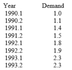
The table below shows semi-annual demand (in 1,000s) for Shidgets (they're like Widgets, only quieter). A linear trend has been estimated using this data set with t = 1 for 1990.1 and t = 8 for 1993.2. It has an intercept of 0.76 and a slope of 0.20. Use the ratio-to-trend method to calculate seasonal adjustment factors for the first and second half of the year and then forecast the level of demand for 1995.1 and 1995.2. Note: round all intermediate calculations to two decimal places.
Question
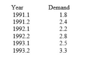
The table below shows semi-annual demand (in 1,000s) for Didgets (they're like Widgets, only they're easier to work). A linear trend has been estimated using this data set with t = 1 for 1991.1 and t = 6 for 1993.2. It has an intercept of 1.66 and a slope of 0.24. Use the ratio-to-trend method to calculate seasonal adjustment factors for the first and second half of the year and then forecast the level of demand for 1996.1 and 1996.2. Note: round all intermediate calculations to two decimal places.
Question
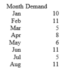
The table below shows the demand for Fidgets (they're like Widgets, only they're more active) over an eight month period. Calculate a four-period moving average forecast for September. Also evaluate the quality of the four-period moving average forecasting model by calculating the root mean square error for the data set. Note: round all intermediate calculations to two decimal places.
Question
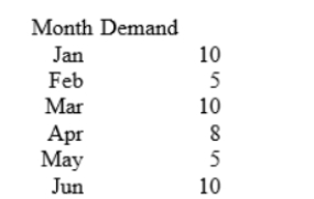
The table below shows the demand for Gadgets (they're like Widgets, only they're more mechanical) over a five-month period. Calculate exponential smoothing forecasts for each month and for July. Use a coefficient of 0.5 and assume that the forecast for January was 8. Also evaluate the quality of the exponential smoothing model by calculating the root-mean-square error for the data set. Note: round all intermediate calculations to two decimal places.
Question
Question

Unlock Deck
Sign up to unlock the cards in this deck!
Unlock Deck
Unlock Deck
1/18
Play
Full screen (f)
Deck 4: Demand Forecasting
1
Regression analysis was used to estimate the following seasonal forecasting equation:
St = 124 + 18 D1 - 46 D2 - 28 D3 + 2.5 t
D1 is a dummy variable that is equal to one in the first quarter and zero otherwise; D2 is a dummy variable that is equal to one in the second quarter and zero otherwise; and D3 is a dummy variable that is equal to one in the third quarter and zero otherwise. Forecast the level of sales in the second quarter of time period ten.
A) 195
B) 170
C) 103
D) None of the above is correct.
103
2
Regression analysis was used to estimate the following seasonal forecasting equation:
St = 124 + 18 D1 - 46 D2 - 28 D3 + 2.5 t
D1 is a dummy variable that is equal to one in the first quarter and zero otherwise; D2 is a dummy variable that is equal to one in the second quarter and zero otherwise; and D3 is a dummy variable that is equal to one in the third quarter and zero otherwise. Forecast the level of sales in the fourth quarter of time period ten.
A) 149
B) 180
C) 205
D) None of the above is correct.
149
3
The Delphi method generates forecasts by surveying consumers to determine their opinions.
False
4
One advantage of the Delphi method is that it avoids a "bandwagon effect"
that could lead to incorrect or biased conclusions.
that could lead to incorrect or biased conclusions.
Unlock Deck
Unlock for access to all 18 flashcards in this deck.
Unlock Deck
k this deck
5
Councils of distinguished foreign dignitaries and businesspersons are used to obtain qualitative forecasts with a foreign perspective.
Unlock Deck
Unlock for access to all 18 flashcards in this deck.
Unlock Deck
k this deck
6
The use of a linear trend equation to forecast future values of a variable is based on the assumption of a constant amount of change per time period.
Unlock Deck
Unlock for access to all 18 flashcards in this deck.
Unlock Deck
k this deck
7
The ratio-to-trend method is used to estimate a linear trend equation.
Unlock Deck
Unlock for access to all 18 flashcards in this deck.
Unlock Deck
k this deck
8
The use of leading indicators to forecast time-series data is an example of econometric forecasting.
Unlock Deck
Unlock for access to all 18 flashcards in this deck.
Unlock Deck
k this deck
9
The use of an estimated demand equation to forecast demand is an example of econometric forecasting.
Unlock Deck
Unlock for access to all 18 flashcards in this deck.
Unlock Deck
k this deck
10
Forecasts based on leading indicators are qualitative.
Unlock Deck
Unlock for access to all 18 flashcards in this deck.
Unlock Deck
k this deck
11
Macroeconomic forecasts are generally based on multiple-equation econometric models.
Unlock Deck
Unlock for access to all 18 flashcards in this deck.
Unlock Deck
k this deck
12
Definitional equations must be estimated using regression analysis.
Unlock Deck
Unlock for access to all 18 flashcards in this deck.
Unlock Deck
k this deck
13
The table below shows semi-annual demand (in 1,000s) for Shidgets (they're like Widgets, only quieter). A linear trend has been estimated using this data set with t = 1 for 1990.1 and t = 8 for 1993.2. It has an intercept of 0.76 and a slope of 0.20. Use the ratio-to-trend method to calculate seasonal adjustment factors for the first and second half of the year and then forecast the level of demand for 1995.1 and 1995.2. Note: round all intermediate calculations to two decimal places.
Unlock Deck
Unlock for access to all 18 flashcards in this deck.
Unlock Deck
k this deck
14
The table below shows semi-annual demand (in 1,000s) for Didgets (they're like Widgets, only they're easier to work). A linear trend has been estimated using this data set with t = 1 for 1991.1 and t = 6 for 1993.2. It has an intercept of 1.66 and a slope of 0.24. Use the ratio-to-trend method to calculate seasonal adjustment factors for the first and second half of the year and then forecast the level of demand for 1996.1 and 1996.2. Note: round all intermediate calculations to two decimal places.
Unlock Deck
Unlock for access to all 18 flashcards in this deck.
Unlock Deck
k this deck
15
The table below shows the demand for Fidgets (they're like Widgets, only they're more active) over an eight month period. Calculate a four-period moving average forecast for September. Also evaluate the quality of the four-period moving average forecasting model by calculating the root mean square error for the data set. Note: round all intermediate calculations to two decimal places.
Unlock Deck
Unlock for access to all 18 flashcards in this deck.
Unlock Deck
k this deck
16
The table below shows the demand for Gadgets (they're like Widgets, only they're more mechanical) over a five-month period. Calculate exponential smoothing forecasts for each month and for July. Use a coefficient of 0.5 and assume that the forecast for January was 8. Also evaluate the quality of the exponential smoothing model by calculating the root-mean-square error for the data set. Note: round all intermediate calculations to two decimal places.
Unlock Deck
Unlock for access to all 18 flashcards in this deck.
Unlock Deck
k this deck
17
A firm has determined that its average level of sales (St) per week in $1,000s during a given year depends on the previous year's level of sales (St-1), the previous year's level of advertising (At-1) per month in $1,000s, and the current year's rate of annual industry growth (Gt) in percentage terms. The firm has also determined that the level of industry growth in the current period depends on the previous period's rate of industry growth (Gt-1) and on current period sales by the firm. During the current period, the firm's level of sales was $100,000, advertising was $40,000, and the rate of growth in the industry was 4%. The firm estimated the following two-equation econometric model:
St = 4 + 0.40 St-1 + 0.10 At-1 + Gt and Gt = 1 + 0.5 Gt-1 + 0.5 St
(i) Formulate a single-equation forecasting equation from this model.
(ii) Forecast the level of sales in the next period.
St = 4 + 0.40 St-1 + 0.10 At-1 + Gt and Gt = 1 + 0.5 Gt-1 + 0.5 St
(i) Formulate a single-equation forecasting equation from this model.
(ii) Forecast the level of sales in the next period.
Unlock Deck
Unlock for access to all 18 flashcards in this deck.
Unlock Deck
k this deck
18
A firm has determined that its average level of sales (St) per week in $1,000s during a given year depends on the previous year's level of sales (St-1), the previous year's level of advertising (At-1) per month in $1,000s, and the current year's rate of annual industry growth (Gt) in percentage terms. The firm has also determined that the level of industry growth in the current period depends on the previous period's rate of industry growth (Gt-1) and on current period sales by the firm. During the current period, the firm's average level of sales was $100,000, advertising was $10,000, and the rate of growth in the industry was 2%. The firm estimated the following two-equation econometric model:
St = 5 + 0.50 St-1 + 0.10 At-1 + 2 Gt and Gt = 0.5 Gt-1 + 0.25 St
(i) Formulate a single-equation forecasting equation from this model.
(ii) Forecast the level of sales in the next period.
St = 5 + 0.50 St-1 + 0.10 At-1 + 2 Gt and Gt = 0.5 Gt-1 + 0.25 St
(i) Formulate a single-equation forecasting equation from this model.
(ii) Forecast the level of sales in the next period.
Unlock Deck
Unlock for access to all 18 flashcards in this deck.
Unlock Deck
k this deck
Unlock Deck
Unlock for access to all 18 flashcards in this deck.


