Deck 12: Simple Linear Regression
Full screen (f)
Question
Question
Question
Question
Question
Question
Question
Question
Question
Question
Question
Question
Question
Question
Question
Question
Question
Question
Question
Question
Question
Question
Question
Question
Question
Question
Question
Question
Instruction 12.5
The managing partner of an advertising agency believes that his company's sales are related to the industry sales. He uses Microsoft Excel's Data Analysis tool to analyse the last four years of quarterly data with the following results:

-Referring to Instruction 12.5,the prediction for a quarter in which X = 120 is Y = ____________.
The managing partner of an advertising agency believes that his company's sales are related to the industry sales. He uses Microsoft Excel's Data Analysis tool to analyse the last four years of quarterly data with the following results:
-Referring to Instruction 12.5,the prediction for a quarter in which X = 120 is Y = ____________.
Question
Question
Question
Question
Question
Instruction 12.7
It is believed that average grade (based on a four-point scale) should have a positive linear relationship with university entrance exam scores. Given below is the Microsoft Excel output from regressing average grade on university entrance exam scores using a data set of eight randomly chosen students from a large university.

-Referring to Instruction 12.7,the interpretation of the coefficient of determination in this regression is
A) average grade accounts for 57.74% of the variability of university entrance exam scores.
B) university entrance exam scores account for 57.74% of the total fluctuation in average grade.
C) 57.74% of the total variation of university entrance exam scores can be explained by average grade.
D) None of the above.
It is believed that average grade (based on a four-point scale) should have a positive linear relationship with university entrance exam scores. Given below is the Microsoft Excel output from regressing average grade on university entrance exam scores using a data set of eight randomly chosen students from a large university.
-Referring to Instruction 12.7,the interpretation of the coefficient of determination in this regression is
A) average grade accounts for 57.74% of the variability of university entrance exam scores.
B) university entrance exam scores account for 57.74% of the total fluctuation in average grade.
C) 57.74% of the total variation of university entrance exam scores can be explained by average grade.
D) None of the above.
Question
Question
Question
Question
Question
Instruction 12.7
It is believed that average grade (based on a four-point scale) should have a positive linear relationship with university entrance exam scores. Given below is the Microsoft Excel output from regressing average grade on university entrance exam scores using a data set of eight randomly chosen students from a large university.
-Referring to Instruction 12.7,what is the predicted average value of average grade when university entrance exam score = 20?
A) 2.80
B) 2.61
C) 2.66
D) 3.12
Question
Question
Instruction 12.5
The managing partner of an advertising agency believes that his company's sales are related to the industry sales. He uses Microsoft Excel's Data Analysis tool to analyse the last four years of quarterly data with the following results:
-Referring to Instruction 12.5,the estimates of the Y-intercept and slope are ____________ and ____________,respectively.
Question
Question
Question
Question
Question
Instruction 12.10
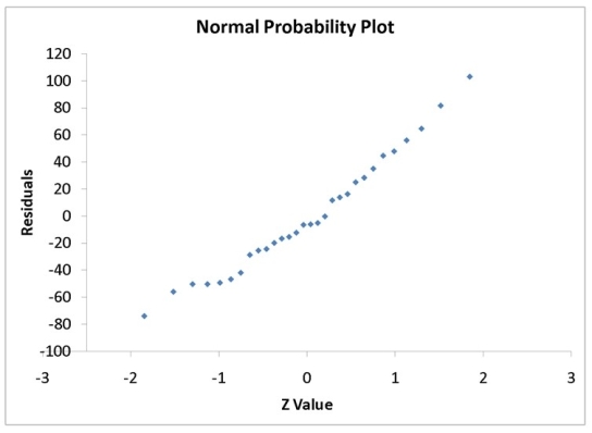
A computer software developer would like to use the number of downloads (in thousands) for the trial version of his new shareware to predict the amount of revenue (in thousands of dollars) he can make on the full version of the new shareware. Following is the output from a simple linear regression along with the residual plot and normal probability plot obtained from a data set of 30 different sharewares that he has developed:
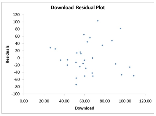
-Referring to Instruction 12.10,which of the following is the correct interpretation for the slope coefficient?
A) For each increase of 1,000 downloads, the expected revenue is estimated to increase by $3.7297 thousands.
B) For each increase of 1,000 dollars in expected revenue, the expected number of downloads is estimated to increase by 3.7297 thousands.
C) For each decrease of 1,000 dollars in expected revenue, the expected number of downloads is estimated to increase by 3.7297 thousands.
D) For each decrease of 1,000 downloads, the expected revenue is estimated to increase by $3.7297 thousands.
A computer software developer would like to use the number of downloads (in thousands) for the trial version of his new shareware to predict the amount of revenue (in thousands of dollars) he can make on the full version of the new shareware. Following is the output from a simple linear regression along with the residual plot and normal probability plot obtained from a data set of 30 different sharewares that he has developed:
-Referring to Instruction 12.10,which of the following is the correct interpretation for the slope coefficient?
A) For each increase of 1,000 downloads, the expected revenue is estimated to increase by $3.7297 thousands.
B) For each increase of 1,000 dollars in expected revenue, the expected number of downloads is estimated to increase by 3.7297 thousands.
C) For each decrease of 1,000 dollars in expected revenue, the expected number of downloads is estimated to increase by 3.7297 thousands.
D) For each decrease of 1,000 downloads, the expected revenue is estimated to increase by $3.7297 thousands.
Question
Question
Question
Question
Question
Instruction 12.10
A computer software developer would like to use the number of downloads (in thousands) for the trial version of his new shareware to predict the amount of revenue (in thousands of dollars) he can make on the full version of the new shareware. Following is the output from a simple linear regression along with the residual plot and normal probability plot obtained from a data set of 30 different sharewares that he has developed:
-Referring to Instruction 12.10,predict the revenue when the number of downloads is 30,000.
Question
Question
Question
Question
Question
Question
Instruction 12.11
The manager of the purchasing department of a large savings and loan organization would like to develop a model to predict the amount of time (measured in hours) it takes to record a loan application. Data are collected from a sample of 30 days, and the number of applications recorded and completion time in hours is recorded. Below is the regression output:
Note: 4.3946E-15 is 4.3946 × 10⁻¹⁵.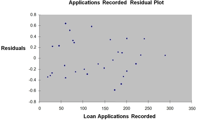
-Referring to Instruction 12.11,the estimated mean amount of time it takes to record one additional loan application is
A) 0.4024 more hours.
B) 0.0126 more hours.
C) 0.0126 fewer hours.
D) 0.4024 fewer hours.
Question
Question
Question
Question
Instruction 12.10
A computer software developer would like to use the number of downloads (in thousands) for the trial version of his new shareware to predict the amount of revenue (in thousands of dollars) he can make on the full version of the new shareware. Following is the output from a simple linear regression along with the residual plot and normal probability plot obtained from a data set of 30 different sharewares that he has developed:
-Referring to Instruction 12.10,which of the following is the correct interpretation for the slope coefficient?
A) For each incsrease of 1 million dollars in box office gross, expected home video units sold are estimated to increase by 4.3331 thousand units.
B) For each increase of 1 dollar in box office gross, expected home video units sold are estimated to increase by 4.3331 units.
C) For each increase of 1 million dollars in box office gross, expected home video units sold are estimated to increase by 4.3331 units.
D) For each increase of 1 dollar in box office gross, expected home video units sold are estimated to increase by 4.3331 thousand units.
Question
Question
Question
Question
Instruction 12.18
The manager of the purchasing department of a large savings and loan organization would like to develop a model to predict the amount of time (measured in hours) it takes to record a loan application. Data are collected from a sample of 30 days, and the number of applications recorded and completion time in hours is recorded. Below is the regression output:
Note: 4.3946E-15 is 4.3946 x 10⁻¹⁵.
 Note: 4.3946E-15 is 4.3946 × 10⁻¹⁵.
-Referring to Instruction 12.18,the error sum of squares (SSE)of the above regression is
A) 0.1117.
B) 29.0720.
C) 25.9438.
D) 3.1282.
The manager of the purchasing department of a large savings and loan organization would like to develop a model to predict the amount of time (measured in hours) it takes to record a loan application. Data are collected from a sample of 30 days, and the number of applications recorded and completion time in hours is recorded. Below is the regression output:
Note: 4.3946E-15 is 4.3946 x 10⁻¹⁵.
Note: 4.3946E-15 is 4.3946 × 10⁻¹⁵.-Referring to Instruction 12.18,the error sum of squares (SSE)of the above regression is
A) 0.1117.
B) 29.0720.
C) 25.9438.
D) 3.1282.
Question
Instruction 12.17
A computer software developer would like to use the number of downloads (in thousands) for the trial version of his new shareware to predict the amount of revenue (in thousands of dollars) he can make on the full version of the new shareware. Following is the output from a simple linear regression along with the residual plot and normal probability plot obtained from a data set of 30 different sharewares that he has developed:


-Referring to Instruction 12.17,which of the following is the correct interpretation for the coefficient of determination?
A) 72.8% of the variation in the video unit sales can be explained by the variation in the box office gross.
B) 71.8% of the variation in the video unit sales can be explained by the variation in the box office gross.
C) 71.8% of the variation in the box office gross can be explained by the variation in the video unit sales.
D) 72.8% of the variation in the box office gross can be explained by the variation in the video unit sales.
A computer software developer would like to use the number of downloads (in thousands) for the trial version of his new shareware to predict the amount of revenue (in thousands of dollars) he can make on the full version of the new shareware. Following is the output from a simple linear regression along with the residual plot and normal probability plot obtained from a data set of 30 different sharewares that he has developed:
-Referring to Instruction 12.17,which of the following is the correct interpretation for the coefficient of determination?
A) 72.8% of the variation in the video unit sales can be explained by the variation in the box office gross.
B) 71.8% of the variation in the video unit sales can be explained by the variation in the box office gross.
C) 71.8% of the variation in the box office gross can be explained by the variation in the video unit sales.
D) 72.8% of the variation in the box office gross can be explained by the variation in the video unit sales.
Question
Question
Question
Question
Instruction 12.17
A computer software developer would like to use the number of downloads (in thousands) for the trial version of his new shareware to predict the amount of revenue (in thousands of dollars) he can make on the full version of the new shareware. Following is the output from a simple linear regression along with the residual plot and normal probability plot obtained from a data set of 30 different sharewares that he has developed:
-Referring to Instruction 12.17,what is the standard deviation around the regression line?
Question
Instruction 12.17
A computer software developer would like to use the number of downloads (in thousands) for the trial version of his new shareware to predict the amount of revenue (in thousands of dollars) he can make on the full version of the new shareware. Following is the output from a simple linear regression along with the residual plot and normal probability plot obtained from a data set of 30 different sharewares that he has developed:
-Referring to Instruction 12.17,which of the following is the correct interpretation for the coefficient of determination?
A) 74.67% of the variation in revenue can be explained by the variation in the number of downloads.
B) 75.54% of the variation in revenue can be explained by the variation in the number of downloads.
C) 75.54% of the variation in the number of downloads can be explained by the variation in revenue.
D) 74.67% of the variation in the number of downloads can be explained by the variation in revenue.
Question
Question
Question
Question
Question
Question
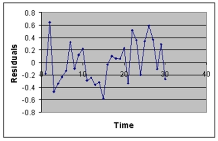
Based on the residual plot below,you will conclude that there might be a violation of which of the following assumptions? 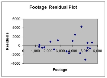
A) Homoscedasticity
B) Independence of errors
C) Linearity of the relationship
D) Normality of errors
A) Homoscedasticity
B) Independence of errors
C) Linearity of the relationship
D) Normality of errors
Question
Instruction 12.17
A computer software developer would like to use the number of downloads (in thousands) for the trial version of his new shareware to predict the amount of revenue (in thousands of dollars) he can make on the full version of the new shareware. Following is the output from a simple linear regression along with the residual plot and normal probability plot obtained from a data set of 30 different sharewares that he has developed:
-Referring to Instruction 12.17,what is the standard error of estimate?
Question
Question
Question

Unlock Deck
Sign up to unlock the cards in this deck!
Unlock Deck
Unlock Deck
1/207
Play
Full screen (f)
Deck 12: Simple Linear Regression
1
Instruction 12.2
A chocolate bar manufacturer is interested in trying to estimate how sales are influenced by the price of their product. To do this, the company randomly chooses six country towns and cities and offers the chocolate bar at different prices. Using chocolate bar sales as the dependent variable, the company will conduct a simple linear regression on the data below:
-Referring to Instruction 12.2,what is the standard error of the regression slope estimate, ?
A) 0.885
B) 12.650
C) 16.299
D) 0.784
12.650
2
A large national bank charges local companies for using their services. A bank official reported the results of a regression analysis designed to predict the bank's charges (Y) - measured in dollars per month - for services rendered to local companies. One independent variable used to predict service charge to a company is the company's sales revenue (X) - measured in millions of dollars. Data for 21 companies who use the bank's services were used to fit the model:
The results of the simple linear regression are provided below:
-Referring to Instruction 12.1,a 95% confidence interval for ?1 is (15,30).Interpret the interval.
A) At the ? = 0.05 level, there is no evidence of a linear relationship between service charge (Y) and sales revenue (X).
B) We are 95% confident that average service charge (Y) will increase between $15 and $30 for every $1 million increase in sales revenue (X).
C) We are 95% confident that the mean service charge will fall between $15 and $30 per month.
D) We are 95% confident that the sales revenue (X) will increase between $15 and $30 million for every $1 increase in service charge (Y).
We are 95% confident that average service charge (Y) will increase between $15 and $30 for every $1 million increase in sales revenue (X).
3
A large national bank charges local companies for using their services. A bank official reported the results of a regression analysis designed to predict the bank's charges (Y) - measured in dollars per month - for services rendered to local companies. One independent variable used to predict service charge to a company is the company's sales revenue (X) - measured in millions of dollars. Data for 21 companies who use the bank's services were used to fit the model:
The results of the simple linear regression are provided below:
-Referring to Instruction 12.1,interpret the p-value for testing whether ?1 exceeds 0.
A) There is sufficient evidence (at the ? = 0.05) to conclude that sales revenue (X) is a useful linear predictor of service charge (Y).
B) Sales revenue (X) is a poor predictor of service charge (Y).
C) There is insufficient evidence (at the ? = 0.10) to conclude that sales revenue (X) is a useful linear predictor of service charge (Y).
D) For every $1 million increase in sales revenue, we expect a service charge to increase $0.034.
There is sufficient evidence (at the ? = 0.05) to conclude that sales revenue (X) is a useful linear predictor of service charge (Y).
4
Instruction 12.2
A chocolate bar manufacturer is interested in trying to estimate how sales are influenced by the price of their product. To do this, the company randomly chooses six country towns and cities and offers the chocolate bar at different prices. Using chocolate bar sales as the dependent variable, the company will conduct a simple linear regression on the data below:
-Referring to Instruction 12.2,to test whether a change in price will have any impact on average sales,what would be the critical values? Use ? = 0.05.
A) ± 2.7765
B) ± 3.1634
C) ± 2.5706
D) ± 3.4954
Unlock Deck
Unlock for access to all 207 flashcards in this deck.
Unlock Deck
k this deck
5
Instruction 12.2
A chocolate bar manufacturer is interested in trying to estimate how sales are influenced by the price of their product. To do this, the company randomly chooses six country towns and cities and offers the chocolate bar at different prices. Using chocolate bar sales as the dependent variable, the company will conduct a simple linear regression on the data below:
-Referring to Instruction 12.2,what is the coefficient of correlation for these data?
A) 0.8854
B) 0.7839
C) -0.7839
D) -0.8854
Unlock Deck
Unlock for access to all 207 flashcards in this deck.
Unlock Deck
k this deck
6
Instruction 12.2
A chocolate bar manufacturer is interested in trying to estimate how sales are influenced by the price of their product. To do this, the company randomly chooses six country towns and cities and offers the chocolate bar at different prices. Using chocolate bar sales as the dependent variable, the company will conduct a simple linear regression on the data below:
-Referring to Instruction 12.2,if the price of the chocolate bar is set at $2,the predicted sales will be
A) 100.
B) 30.
C) 65.
D) 90.
Unlock Deck
Unlock for access to all 207 flashcards in this deck.
Unlock Deck
k this deck
7
Instruction 12.3
The director of cooperative education at a university wants to examine the effect of cooperative education job experience on marketability in the workplace. She takes a random sample of four students. For these four, she finds out how many times each had a cooperative education job and how many job offers they received upon graduation. These data are presented in the table below.
-Referring to Instruction 12.3,the prediction for the number of job offers for a person with two cooperative jobs is____________.
Unlock Deck
Unlock for access to all 207 flashcards in this deck.
Unlock Deck
k this deck
8
Instruction 12.3
The director of cooperative education at a university wants to examine the effect of cooperative education job experience on marketability in the workplace. She takes a random sample of four students. For these four, she finds out how many times each had a cooperative education job and how many job offers they received upon graduation. These data are presented in the table below.
-Referring to Instruction 12.3,the total sum of squares (SST)is ____________.
Unlock Deck
Unlock for access to all 207 flashcards in this deck.
Unlock Deck
k this deck
9
A large national bank charges local companies for using their services. A bank official reported the results of a regression analysis designed to predict the bank's charges (Y) - measured in dollars per month - for services rendered to local companies. One independent variable used to predict service charge to a company is the company's sales revenue (X) - measured in millions of dollars. Data for 21 companies who use the bank's services were used to fit the model:
The results of the simple linear regression are provided below:
-Referring to Instruction 12.1,interpret the estimate of ?0,the Y-intercept of the line.
A) About 95% of the observed service charges fall within $2,700 of the least squares line.
B) There is no practical interpretation since a sales revenue of $0 is a nonsensical value.
C) For every $1 million increase in sales revenue, we expect a service charge to decrease $2,700.
D) All companies will be charged at least $2,700 by the bank.
Unlock Deck
Unlock for access to all 207 flashcards in this deck.
Unlock Deck
k this deck
10
Instruction 12.2
A chocolate bar manufacturer is interested in trying to estimate how sales are influenced by the price of their product. To do this, the company randomly chooses six country towns and cities and offers the chocolate bar at different prices. Using chocolate bar sales as the dependent variable, the company will conduct a simple linear regression on the data below:
-Referring to Instruction 12.2,what is the standard error of the estimate,SYX,for the data?
A) 0.885
B) 0.784
C) 16.299
D) 12.650
Unlock Deck
Unlock for access to all 207 flashcards in this deck.
Unlock Deck
k this deck
11
Instruction 12.2
A chocolate bar manufacturer is interested in trying to estimate how sales are influenced by the price of their product. To do this, the company randomly chooses six country towns and cities and offers the chocolate bar at different prices. Using chocolate bar sales as the dependent variable, the company will conduct a simple linear regression on the data below:
-Referring to Instruction 12.2,what percentage of the total variation in chocolate bar sales is explained by prices?
A) 78.39%
B) 88.54%
C) 48.19%
D) 100%
Unlock Deck
Unlock for access to all 207 flashcards in this deck.
Unlock Deck
k this deck
12
Instruction 12.2
A chocolate bar manufacturer is interested in trying to estimate how sales are influenced by the price of their product. To do this, the company randomly chooses six country towns and cities and offers the chocolate bar at different prices. Using chocolate bar sales as the dependent variable, the company will conduct a simple linear regression on the data below:
-Referring to Instruction 12.2,what is ?(X * )2 for these data?
A) 25.66
B) 0
C) 2.54
D) 1.66
Unlock Deck
Unlock for access to all 207 flashcards in this deck.
Unlock Deck
k this deck
13
Instruction 12.2
A chocolate bar manufacturer is interested in trying to estimate how sales are influenced by the price of their product. To do this, the company randomly chooses six country towns and cities and offers the chocolate bar at different prices. Using chocolate bar sales as the dependent variable, the company will conduct a simple linear regression on the data below:
-Referring to Instruction 12.2,what is the percentage of the total variation in chocolate bar sales explained by the regression model?
A) 48.19%
B) 100%
C) 88.54%
D) 78.39%
Unlock Deck
Unlock for access to all 207 flashcards in this deck.
Unlock Deck
k this deck
14
Instruction 12.3
The director of cooperative education at a university wants to examine the effect of cooperative education job experience on marketability in the workplace. She takes a random sample of four students. For these four, she finds out how many times each had a cooperative education job and how many job offers they received upon graduation. These data are presented in the table below.
-Referring to Instruction 12.3,the least squares estimate of the Y-intercept is____________.
Unlock Deck
Unlock for access to all 207 flashcards in this deck.
Unlock Deck
k this deck
15
Instruction 12.2
A chocolate bar manufacturer is interested in trying to estimate how sales are influenced by the price of their product. To do this, the company randomly chooses six country towns and cities and offers the chocolate bar at different prices. Using chocolate bar sales as the dependent variable, the company will conduct a simple linear regression on the data below:
-Referring to Instruction 12.2,what is the estimated average change in the sales of the chocolate bar if price goes up by $1.00?
A) 0.784
B) -3.810
C) 161.386
D) -48.193
Unlock Deck
Unlock for access to all 207 flashcards in this deck.
Unlock Deck
k this deck
16
Instruction 12.2
A chocolate bar manufacturer is interested in trying to estimate how sales are influenced by the price of their product. To do this, the company randomly chooses six country towns and cities and offers the chocolate bar at different prices. Using chocolate bar sales as the dependent variable, the company will conduct a simple linear regression on the data below:
-Referring to Instruction 12.2,to test that the regression coefficient,?1 is not equal to 0,what would be the critical values? Use ? = 0.05.
A) ± 2.7765
B) ± 3.1634
C) ± 2.5706
D) ± 3.4954
Unlock Deck
Unlock for access to all 207 flashcards in this deck.
Unlock Deck
k this deck
17
Instruction 12.3
The director of cooperative education at a university wants to examine the effect of cooperative education job experience on marketability in the workplace. She takes a random sample of four students. For these four, she finds out how many times each had a cooperative education job and how many job offers they received upon graduation. These data are presented in the table below.
-Referring to Instruction 12.3,the least squares estimate of the slope is_____________.
Unlock Deck
Unlock for access to all 207 flashcards in this deck.
Unlock Deck
k this deck
18
Instruction 12.2
A chocolate bar manufacturer is interested in trying to estimate how sales are influenced by the price of their product. To do this, the company randomly chooses six country towns and cities and offers the chocolate bar at different prices. Using chocolate bar sales as the dependent variable, the company will conduct a simple linear regression on the data below:
-Referring to Instruction 12.2,what is the estimated slope parameter for the chocolate bar price and sales data?
A) -48.193
B) -3.810
C) 161.386
D) 0.784
Unlock Deck
Unlock for access to all 207 flashcards in this deck.
Unlock Deck
k this deck
19
A large national bank charges local companies for using their services. A bank official reported the results of a regression analysis designed to predict the bank's charges (Y) - measured in dollars per month - for services rendered to local companies. One independent variable used to predict service charge to a company is the company's sales revenue (X) - measured in millions of dollars. Data for 21 companies who use the bank's services were used to fit the model:
The results of the simple linear regression are provided below:
-Referring to Instruction 12.1,interpret the estimate of ?,the standard deviation of the random error term (standard error of the estimate)in the model.
A) About 95% of the observed service charges fall within $130 of the least squares line.
B) About 95% of the observed service charges fall within $65 of the least squares line.
C) About 95% of the observed service charges equal their corresponding predicted values.
D) For every $1 million increase in sales revenue, we expect a service charge to increase $65.
Unlock Deck
Unlock for access to all 207 flashcards in this deck.
Unlock Deck
k this deck
20
Instruction 12.3
The director of cooperative education at a university wants to examine the effect of cooperative education job experience on marketability in the workplace. She takes a random sample of four students. For these four, she finds out how many times each had a cooperative education job and how many job offers they received upon graduation. These data are presented in the table below.
-Referring to Instruction 12.3,the regression sum of squares (SSR)is____________.
Unlock Deck
Unlock for access to all 207 flashcards in this deck.
Unlock Deck
k this deck
21
Instruction 12.4
The managers of a brokerage firm are interested in finding out if the number of new customers a broker brings into the firm affects the sales generated by the broker. They sample 12 brokers and determine the number of new customers they have enrolled in the last year and their sales amounts in thousands of dollars. These data are presented in the table that follows.
-Referring to Instruction 12.4,the regression sum of squares (SSR)is____________
Unlock Deck
Unlock for access to all 207 flashcards in this deck.
Unlock Deck
k this deck
22
Instruction 12.9
The management of a chain electronic store would like to develop a model for predicting the weekly sales (in thousands of dollars) for individual stores based on the number of customers who made purchases. A random sample of 12 stores yields the following results:
-Referring to Instruction 12.9,93.98% of the total variation in weekly sales can be explained by the variation in the number of customers who make purchases.
Unlock Deck
Unlock for access to all 207 flashcards in this deck.
Unlock Deck
k this deck
23
Instruction 12.8
It is believed that the average numbers of hours spent studying per day (HOURS) during undergraduate education should have a positive linear relationship with the starting salary (SALARY, measured in thousands of dollars per month) after graduation. Given below is the Microsoft Excel output for predicting starting salary (Y) using number of hours spent studying per day (X) for a sample of 51 students. NOTE: Only partial output is shown.
Note: 2.051E-05 = 2.051 * 10S1-0.5 and 5.944E-18 = 5.944 * 10S1-18.
-Referring to Instruction 12.8,the estimated average change in salary (in thousands of dollars)as a result of spending an extra hour per day studying is
A) 0.9795.
B) 0.7845.
C) 335.0473.
D) -1.8940.
Unlock Deck
Unlock for access to all 207 flashcards in this deck.
Unlock Deck
k this deck
24
Instruction 12.9
The management of a chain electronic store would like to develop a model for predicting the weekly sales (in thousands of dollars) for individual stores based on the number of customers who made purchases. A random sample of 12 stores yields the following results:
-Referring to Instruction 12.9,generate the scatter plot.
Unlock Deck
Unlock for access to all 207 flashcards in this deck.
Unlock Deck
k this deck
25
Instruction 12.9
The management of a chain electronic store would like to develop a model for predicting the weekly sales (in thousands of dollars) for individual stores based on the number of customers who made purchases. A random sample of 12 stores yields the following results:
-Referring to Instruction 12.9,what are the values of the estimated intercept and slope?
Unlock Deck
Unlock for access to all 207 flashcards in this deck.
Unlock Deck
k this deck
26
Instruction 12.4
The managers of a brokerage firm are interested in finding out if the number of new customers a broker brings into the firm affects the sales generated by the broker. They sample 12 brokers and determine the number of new customers they have enrolled in the last year and their sales amounts in thousands of dollars. These data are presented in the table that follows.
-Referring to Instruction 12.4,the total sum of squares (SST)is ____________.
Unlock Deck
Unlock for access to all 207 flashcards in this deck.
Unlock Deck
k this deck
27
Instruction 12.4
The managers of a brokerage firm are interested in finding out if the number of new customers a broker brings into the firm affects the sales generated by the broker. They sample 12 brokers and determine the number of new customers they have enrolled in the last year and their sales amounts in thousands of dollars. These data are presented in the table that follows.
-Referring to Instruction 12.4,the prediction for the amount of sales (in $1,000s)for a person who brings 25 new customers into the firm is ____________.
Unlock Deck
Unlock for access to all 207 flashcards in this deck.
Unlock Deck
k this deck
28
Instruction 12.5
The managing partner of an advertising agency believes that his company's sales are related to the industry sales. He uses Microsoft Excel's Data Analysis tool to analyse the last four years of quarterly data with the following results:
-Referring to Instruction 12.5,the prediction for a quarter in which X = 120 is Y = ____________.
Unlock Deck
Unlock for access to all 207 flashcards in this deck.
Unlock Deck
k this deck
29
Instruction 12.3
The director of cooperative education at a university wants to examine the effect of cooperative education job experience on marketability in the workplace. She takes a random sample of four students. For these four, she finds out how many times each had a cooperative education job and how many job offers they received upon graduation. These data are presented in the table below.
-Referring to Instruction 12.3,set up a scatter diagram.
Unlock Deck
Unlock for access to all 207 flashcards in this deck.
Unlock Deck
k this deck
30
Instruction 12.3
The director of cooperative education at a university wants to examine the effect of cooperative education job experience on marketability in the workplace. She takes a random sample of four students. For these four, she finds out how many times each had a cooperative education job and how many job offers they received upon graduation. These data are presented in the table below.
-Referring to Instruction 12.3,the coefficient of determination is____________.
Unlock Deck
Unlock for access to all 207 flashcards in this deck.
Unlock Deck
k this deck
31
Instruction 12.4
The managers of a brokerage firm are interested in finding out if the number of new customers a broker brings into the firm affects the sales generated by the broker. They sample 12 brokers and determine the number of new customers they have enrolled in the last year and their sales amounts in thousands of dollars. These data are presented in the table that follows.
-Referring to Instruction 12.4,the least squares estimate of the Y-intercept is ____________.
Unlock Deck
Unlock for access to all 207 flashcards in this deck.
Unlock Deck
k this deck
32
Instruction 12.4
The managers of a brokerage firm are interested in finding out if the number of new customers a broker brings into the firm affects the sales generated by the broker. They sample 12 brokers and determine the number of new customers they have enrolled in the last year and their sales amounts in thousands of dollars. These data are presented in the table that follows.
-Referring to Instruction 12.4,the error or residual sum of squares (SSE)is____________.
Unlock Deck
Unlock for access to all 207 flashcards in this deck.
Unlock Deck
k this deck
33
Instruction 12.7
It is believed that average grade (based on a four-point scale) should have a positive linear relationship with university entrance exam scores. Given below is the Microsoft Excel output from regressing average grade on university entrance exam scores using a data set of eight randomly chosen students from a large university.
-Referring to Instruction 12.7,the interpretation of the coefficient of determination in this regression is
A) average grade accounts for 57.74% of the variability of university entrance exam scores.
B) university entrance exam scores account for 57.74% of the total fluctuation in average grade.
C) 57.74% of the total variation of university entrance exam scores can be explained by average grade.
D) None of the above.
Unlock Deck
Unlock for access to all 207 flashcards in this deck.
Unlock Deck
k this deck
34
Instruction 12.4
The managers of a brokerage firm are interested in finding out if the number of new customers a broker brings into the firm affects the sales generated by the broker. They sample 12 brokers and determine the number of new customers they have enrolled in the last year and their sales amounts in thousands of dollars. These data are presented in the table that follows.
-Referring to Instruction 12.4,set up a scatter diagram.
Unlock Deck
Unlock for access to all 207 flashcards in this deck.
Unlock Deck
k this deck
35
Instruction 12.4
The managers of a brokerage firm are interested in finding out if the number of new customers a broker brings into the firm affects the sales generated by the broker. They sample 12 brokers and determine the number of new customers they have enrolled in the last year and their sales amounts in thousands of dollars. These data are presented in the table that follows.
-Referring to Instruction 12.4,____% of the total variation in sales generated can be explained by the number of new customers brought in.
Unlock Deck
Unlock for access to all 207 flashcards in this deck.
Unlock Deck
k this deck
36
Instruction 12.6
The following Microsoft Excel tables are obtained when 'Score received on an exam (measured in percentage points)' (Y) is regressed on 'percentage attendance' (X) for 22 students in a Statistics for Business and Economics course.
-Referring to Instruction 12.6,which of the following statements is true?
A) If attendance increases by 1%, the estimated mean score received will increase by 39.39 percentage points.
B) If attendance increases by 0.341%, the estimated mean score received will increase by 1 percentage point.
C) If the score received increases by 39.39%, the estimated mean attendance will go up by 1%.
D) If attendance increases by 1%, the estimated mean score received will increase by 0.341 percentage points.
Unlock Deck
Unlock for access to all 207 flashcards in this deck.
Unlock Deck
k this deck
37
Instruction 12.8
It is believed that the average numbers of hours spent studying per day (HOURS) during undergraduate education should have a positive linear relationship with the starting salary (SALARY, measured in thousands of dollars per month) after graduation. Given below is the Microsoft Excel output for predicting starting salary (Y) using number of hours spent studying per day (X) for a sample of 51 students. NOTE: Only partial output is shown.
Note: 2.051E-05 = 2.051 * 10S1-0.5 and 5.944E-18 = 5.944 * 10S1-18.
-Referring to Instruction 12.8,the error sum of squares (SSE)of the above regression is
A) 427.079804.
B) 92.0325465.
C) 1.878215.
D) 335.047257.
Unlock Deck
Unlock for access to all 207 flashcards in this deck.
Unlock Deck
k this deck
38
Instruction 12.7
It is believed that average grade (based on a four-point scale) should have a positive linear relationship with university entrance exam scores. Given below is the Microsoft Excel output from regressing average grade on university entrance exam scores using a data set of eight randomly chosen students from a large university.
-Referring to Instruction 12.7,what is the predicted average value of average grade when university entrance exam score = 20?
A) 2.80
B) 2.61
C) 2.66
D) 3.12
Unlock Deck
Unlock for access to all 207 flashcards in this deck.
Unlock Deck
k this deck
39
Instruction 12.3
The director of cooperative education at a university wants to examine the effect of cooperative education job experience on marketability in the workplace. She takes a random sample of four students. For these four, she finds out how many times each had a cooperative education job and how many job offers they received upon graduation. These data are presented in the table below.
-Referring to Instruction 12.3,the error or residual sum of squares (SSE)is____________.
Unlock Deck
Unlock for access to all 207 flashcards in this deck.
Unlock Deck
k this deck
40
Instruction 12.5
The managing partner of an advertising agency believes that his company's sales are related to the industry sales. He uses Microsoft Excel's Data Analysis tool to analyse the last four years of quarterly data with the following results:
-Referring to Instruction 12.5,the estimates of the Y-intercept and slope are ____________ and ____________,respectively.
Unlock Deck
Unlock for access to all 207 flashcards in this deck.
Unlock Deck
k this deck
41
When using a regression model to make predictions,the term 'relevant range' refers to____________.
Unlock Deck
Unlock for access to all 207 flashcards in this deck.
Unlock Deck
k this deck
42
The standard error of the estimate is a measure of
A) total variation of the Y variable.
B) explained variation.
C) the variation of the X variable.
D) the variation around the sample regression line.
A) total variation of the Y variable.
B) explained variation.
C) the variation of the X variable.
D) the variation around the sample regression line.
Unlock Deck
Unlock for access to all 207 flashcards in this deck.
Unlock Deck
k this deck
43
What do we mean when we say that a simple linear regression model is 'statistically' useful?
A) The model is 'practically' useful for predicting Y.
B) The model is an excellent predictor of Y.
C) All the statistics computed from the sample make sense.
D) The model is a better predictor of Y than the sample mean, .
A) The model is 'practically' useful for predicting Y.
B) The model is an excellent predictor of Y.
C) All the statistics computed from the sample make sense.
D) The model is a better predictor of Y than the sample mean, .
Unlock Deck
Unlock for access to all 207 flashcards in this deck.
Unlock Deck
k this deck
44
A simple regression has a b0 value of 5 and a b1 value of 3.5.What is the predicted Y for an X value of -2?
A) 13.5
B) 12.0
C) -6.0
D) -2.0
A) 13.5
B) 12.0
C) -6.0
D) -2.0
Unlock Deck
Unlock for access to all 207 flashcards in this deck.
Unlock Deck
k this deck
45
Instruction 12.10
A computer software developer would like to use the number of downloads (in thousands) for the trial version of his new shareware to predict the amount of revenue (in thousands of dollars) he can make on the full version of the new shareware. Following is the output from a simple linear regression along with the residual plot and normal probability plot obtained from a data set of 30 different sharewares that he has developed:
-Referring to Instruction 12.10,which of the following is the correct interpretation for the slope coefficient?
A) For each increase of 1,000 downloads, the expected revenue is estimated to increase by $3.7297 thousands.
B) For each increase of 1,000 dollars in expected revenue, the expected number of downloads is estimated to increase by 3.7297 thousands.
C) For each decrease of 1,000 dollars in expected revenue, the expected number of downloads is estimated to increase by 3.7297 thousands.
D) For each decrease of 1,000 downloads, the expected revenue is estimated to increase by $3.7297 thousands.
Unlock Deck
Unlock for access to all 207 flashcards in this deck.
Unlock Deck
k this deck
46
The slope (b1)represents
A) the estimated average change in Y per unit change in X.
B) predicted value of Y when X = 0.
C) variation around the line of regression.
D) the predicted value of Y.
A) the estimated average change in Y per unit change in X.
B) predicted value of Y when X = 0.
C) variation around the line of regression.
D) the predicted value of Y.
Unlock Deck
Unlock for access to all 207 flashcards in this deck.
Unlock Deck
k this deck
47
The regression sum of squares (SSR)can never be greater than the total sum of squares (SST).
Unlock Deck
Unlock for access to all 207 flashcards in this deck.
Unlock Deck
k this deck
48
When using a regression model to make predictions,you should not predict Y for values of X larger or smaller than the values used to develop the model.
Unlock Deck
Unlock for access to all 207 flashcards in this deck.
Unlock Deck
k this deck
49
A simple regression has a b0 value of 1.3 and a b1 value of 2.6.What is the predicted Y for an X value of 0?
A) 2.6
B) 3.9
C) 1.3
D) 3.4
A) 2.6
B) 3.9
C) 1.3
D) 3.4
Unlock Deck
Unlock for access to all 207 flashcards in this deck.
Unlock Deck
k this deck
50
Instruction 12.10
A computer software developer would like to use the number of downloads (in thousands) for the trial version of his new shareware to predict the amount of revenue (in thousands of dollars) he can make on the full version of the new shareware. Following is the output from a simple linear regression along with the residual plot and normal probability plot obtained from a data set of 30 different sharewares that he has developed:
-Referring to Instruction 12.10,predict the revenue when the number of downloads is 30,000.
Unlock Deck
Unlock for access to all 207 flashcards in this deck.
Unlock Deck
k this deck
51
The coefficient of determination (r2)tells you
A) the proportion of variation in Y that is explained by the independent variable X in the model.
B) whether r has any significance.
C) that you should not partition the total variation.
D) that the coefficient of correlation (r) is larger than 1.
A) the proportion of variation in Y that is explained by the independent variable X in the model.
B) whether r has any significance.
C) that you should not partition the total variation.
D) that the coefficient of correlation (r) is larger than 1.
Unlock Deck
Unlock for access to all 207 flashcards in this deck.
Unlock Deck
k this deck
52
The least squares method minimises which of the following?
A) SST
B) SSR
C) SSE
D) All of the above.
A) SST
B) SSR
C) SSE
D) All of the above.
Unlock Deck
Unlock for access to all 207 flashcards in this deck.
Unlock Deck
k this deck
53
Instruction 12.12
The director of cooperative education at a university wants to examine the effect of cooperative education job experience on marketability in the workplace. She takes a random sample of four students. For these four, she finds out how many times each had a cooperative education job and how many job offers they received upon graduation. These data are presented in the table below.
-Referring to Instruction 12.12,the standard error of estimate is ____________.
Unlock Deck
Unlock for access to all 207 flashcards in this deck.
Unlock Deck
k this deck
54
Instruction 12.13
The managers of a brokerage firm are interested in finding out if the number of new customers a broker brings into the firm affects the sales generated by the broker. They sample 12 brokers and determine the number of new customers they have enrolled in the last year and their sales amounts in thousands of dollars. These data are presented in the table that follows.
-Referring to Instruction 12.13,the coefficient of determination is ____________.
Unlock Deck
Unlock for access to all 207 flashcards in this deck.
Unlock Deck
k this deck
55
The coefficient of determination represents the ratio of SSR to SST.
Unlock Deck
Unlock for access to all 207 flashcards in this deck.
Unlock Deck
k this deck
56
Instruction 12.11
The manager of the purchasing department of a large savings and loan organization would like to develop a model to predict the amount of time (measured in hours) it takes to record a loan application. Data are collected from a sample of 30 days, and the number of applications recorded and completion time in hours is recorded. Below is the regression output:
Note: 4.3946E-15 is 4.3946 × 10⁻¹⁵.
-Referring to Instruction 12.11,the estimated mean amount of time it takes to record one additional loan application is
A) 0.4024 more hours.
B) 0.0126 more hours.
C) 0.0126 fewer hours.
D) 0.4024 fewer hours.
The manager of the purchasing department of a large savings and loan organization would like to develop a model to predict the amount of time (measured in hours) it takes to record a loan application. Data are collected from a sample of 30 days, and the number of applications recorded and completion time in hours is recorded. Below is the regression output:
Note: 4.3946E-15 is 4.3946 × 10⁻¹⁵.
-Referring to Instruction 12.11,the estimated mean amount of time it takes to record one additional loan application is
A) 0.4024 more hours.
B) 0.0126 more hours.
C) 0.0126 fewer hours.
D) 0.4024 fewer hours.
Unlock Deck
Unlock for access to all 207 flashcards in this deck.
Unlock Deck
k this deck
57
The Y-intercept (b0)represents the
A) predicted value of Y.
B) change in estimated average Y per unit change in X.
C) estimated average Y when X = 0.
D) variation around the sample regression line.
A) predicted value of Y.
B) change in estimated average Y per unit change in X.
C) estimated average Y when X = 0.
D) variation around the sample regression line.
Unlock Deck
Unlock for access to all 207 flashcards in this deck.
Unlock Deck
k this deck
58
Instruction 12.12
The director of cooperative education at a university wants to examine the effect of cooperative education job experience on marketability in the workplace. She takes a random sample of four students. For these four, she finds out how many times each had a cooperative education job and how many job offers they received upon graduation. These data are presented in the table below.
-Referring to Instruction 12.12,the coefficient of correlation is ____________.
Unlock Deck
Unlock for access to all 207 flashcards in this deck.
Unlock Deck
k this deck
59
Instruction 12.13
The managers of a brokerage firm are interested in finding out if the number of new customers a broker brings into the firm affects the sales generated by the broker. They sample 12 brokers and determine the number of new customers they have enrolled in the last year and their sales amounts in thousands of dollars. These data are presented in the table that follows.
-Referring to Instruction 12.13,the standard error of the estimated slope coefficient is ____________.
Unlock Deck
Unlock for access to all 207 flashcards in this deck.
Unlock Deck
k this deck
60
Instruction 12.10
A computer software developer would like to use the number of downloads (in thousands) for the trial version of his new shareware to predict the amount of revenue (in thousands of dollars) he can make on the full version of the new shareware. Following is the output from a simple linear regression along with the residual plot and normal probability plot obtained from a data set of 30 different sharewares that he has developed:
-Referring to Instruction 12.10,which of the following is the correct interpretation for the slope coefficient?
A) For each incsrease of 1 million dollars in box office gross, expected home video units sold are estimated to increase by 4.3331 thousand units.
B) For each increase of 1 dollar in box office gross, expected home video units sold are estimated to increase by 4.3331 units.
C) For each increase of 1 million dollars in box office gross, expected home video units sold are estimated to increase by 4.3331 units.
D) For each increase of 1 dollar in box office gross, expected home video units sold are estimated to increase by 4.3331 thousand units.
Unlock Deck
Unlock for access to all 207 flashcards in this deck.
Unlock Deck
k this deck
61
Instruction 12.16
The management of a chain electronic store would like to develop a model for predicting the weekly sales (in thousands of dollars) for individual stores based on the number of customers who made purchases. A random sample of 12 stores yields the following results:
-Referring to Instruction 12.16,what is the value of the standard error of the estimate?
Unlock Deck
Unlock for access to all 207 flashcards in this deck.
Unlock Deck
k this deck
62
Instruction 12.14
The managing partner of an advertising agency believes that his company's sales are related to the industry sales. He uses Microsoft Excel's Data Analysis tool to analyse the last four years of quarterly data with the following results:
-Referring to Instruction 12.14,the standard error of the estimated slope coefficient is ____________.
Unlock Deck
Unlock for access to all 207 flashcards in this deck.
Unlock Deck
k this deck
63
Instruction 12.13
The managers of a brokerage firm are interested in finding out if the number of new customers a broker brings into the firm affects the sales generated by the broker. They sample 12 brokers and determine the number of new customers they have enrolled in the last year and their sales amounts in thousands of dollars. These data are presented in the table that follows.
-Referring to Instruction 12.13,the coefficient of correlation is____________.
Unlock Deck
Unlock for access to all 207 flashcards in this deck.
Unlock Deck
k this deck
64
Instruction 12.18
The manager of the purchasing department of a large savings and loan organization would like to develop a model to predict the amount of time (measured in hours) it takes to record a loan application. Data are collected from a sample of 30 days, and the number of applications recorded and completion time in hours is recorded. Below is the regression output:
Note: 4.3946E-15 is 4.3946 x 10⁻¹⁵. Note: 4.3946E-15 is 4.3946 × 10⁻¹⁵.
-Referring to Instruction 12.18,the error sum of squares (SSE)of the above regression is
A) 0.1117.
B) 29.0720.
C) 25.9438.
D) 3.1282.
The manager of the purchasing department of a large savings and loan organization would like to develop a model to predict the amount of time (measured in hours) it takes to record a loan application. Data are collected from a sample of 30 days, and the number of applications recorded and completion time in hours is recorded. Below is the regression output:
Note: 4.3946E-15 is 4.3946 x 10⁻¹⁵.
Note: 4.3946E-15 is 4.3946 × 10⁻¹⁵.-Referring to Instruction 12.18,the error sum of squares (SSE)of the above regression is
A) 0.1117.
B) 29.0720.
C) 25.9438.
D) 3.1282.
Unlock Deck
Unlock for access to all 207 flashcards in this deck.
Unlock Deck
k this deck
65
Instruction 12.17
A computer software developer would like to use the number of downloads (in thousands) for the trial version of his new shareware to predict the amount of revenue (in thousands of dollars) he can make on the full version of the new shareware. Following is the output from a simple linear regression along with the residual plot and normal probability plot obtained from a data set of 30 different sharewares that he has developed:
-Referring to Instruction 12.17,which of the following is the correct interpretation for the coefficient of determination?
A) 72.8% of the variation in the video unit sales can be explained by the variation in the box office gross.
B) 71.8% of the variation in the video unit sales can be explained by the variation in the box office gross.
C) 71.8% of the variation in the box office gross can be explained by the variation in the video unit sales.
D) 72.8% of the variation in the box office gross can be explained by the variation in the video unit sales.
Unlock Deck
Unlock for access to all 207 flashcards in this deck.
Unlock Deck
k this deck
66
Instruction 12.13
The managers of a brokerage firm are interested in finding out if the number of new customers a broker brings into the firm affects the sales generated by the broker. They sample 12 brokers and determine the number of new customers they have enrolled in the last year and their sales amounts in thousands of dollars. These data are presented in the table that follows.
-Referring to Instruction 12.13,the standard error of estimate is ____________.
Unlock Deck
Unlock for access to all 207 flashcards in this deck.
Unlock Deck
k this deck
67
If the plot of the residuals is fan shaped,which assumption is violated?
A) Homoscedasticity
B) Independence of errors
C) Normality
D) No assumptions are violated, the graph should resemble a fan
A) Homoscedasticity
B) Independence of errors
C) Normality
D) No assumptions are violated, the graph should resemble a fan
Unlock Deck
Unlock for access to all 207 flashcards in this deck.
Unlock Deck
k this deck
68
Instruction 12.14
The managing partner of an advertising agency believes that his company's sales are related to the industry sales. He uses Microsoft Excel's Data Analysis tool to analyse the last four years of quarterly data with the following results:
-Referring to Instruction 12.14,the correlation coefficient is ____________.
Unlock Deck
Unlock for access to all 207 flashcards in this deck.
Unlock Deck
k this deck
69
Instruction 12.17
A computer software developer would like to use the number of downloads (in thousands) for the trial version of his new shareware to predict the amount of revenue (in thousands of dollars) he can make on the full version of the new shareware. Following is the output from a simple linear regression along with the residual plot and normal probability plot obtained from a data set of 30 different sharewares that he has developed:
-Referring to Instruction 12.17,what is the standard deviation around the regression line?
Unlock Deck
Unlock for access to all 207 flashcards in this deck.
Unlock Deck
k this deck
70
Instruction 12.17
A computer software developer would like to use the number of downloads (in thousands) for the trial version of his new shareware to predict the amount of revenue (in thousands of dollars) he can make on the full version of the new shareware. Following is the output from a simple linear regression along with the residual plot and normal probability plot obtained from a data set of 30 different sharewares that he has developed:
-Referring to Instruction 12.17,which of the following is the correct interpretation for the coefficient of determination?
A) 74.67% of the variation in revenue can be explained by the variation in the number of downloads.
B) 75.54% of the variation in revenue can be explained by the variation in the number of downloads.
C) 75.54% of the variation in the number of downloads can be explained by the variation in revenue.
D) 74.67% of the variation in the number of downloads can be explained by the variation in revenue.
Unlock Deck
Unlock for access to all 207 flashcards in this deck.
Unlock Deck
k this deck
71
Which of the following assumptions concerning the probability distribution of the random error term is stated incorrectly?
A) The variance of the distribution increases as X increases.
B) The mean of the distribution is 0.
C) The errors are independent.
D) The distribution is normal.
A) The variance of the distribution increases as X increases.
B) The mean of the distribution is 0.
C) The errors are independent.
D) The distribution is normal.
Unlock Deck
Unlock for access to all 207 flashcards in this deck.
Unlock Deck
k this deck
72
Instruction 12.15
The following Microsoft Excel tables are obtained when 'Score received on an exam (measured in percentage points)' (Y) is regressed on 'percentage attendance' (X) for 22 students in a Statistics for Business and Economics course.
-Referring to Instruction 12.15,which of the following statements is true?
A) 14.2% of the total variability in percentage attendance can be explained by score received.
B) 2% of the total variability in score received can be explained by percentage attendance.
C) 2% of the total variability in percentage attendance can be explained by score received.
D) 14.26% of the total variability in score received can be explained by percentage attendance.
Unlock Deck
Unlock for access to all 207 flashcards in this deck.
Unlock Deck
k this deck
73
Instruction 12.14
The managing partner of an advertising agency believes that his company's sales are related to the industry sales. He uses Microsoft Excel's Data Analysis tool to analyse the last four years of quarterly data with the following results:
-Referring to Instruction 12.14,the standard error of the estimate is____________.
Unlock Deck
Unlock for access to all 207 flashcards in this deck.
Unlock Deck
k this deck
74
Instruction 12.14
The managing partner of an advertising agency believes that his company's sales are related to the industry sales. He uses Microsoft Excel's Data Analysis tool to analyse the last four years of quarterly data with the following results:
-Referring to Instruction 12.14,the coefficient of determination is ____________.
Unlock Deck
Unlock for access to all 207 flashcards in this deck.
Unlock Deck
k this deck
75
The residuals represent
A) the square root of the slope.
B) the difference between the actual Y values and the predicted Y values.
C) the difference between the actual Y values and the mean of Y.
D) the predicted value of Y for the average X value.
A) the square root of the slope.
B) the difference between the actual Y values and the predicted Y values.
C) the difference between the actual Y values and the mean of Y.
D) the predicted value of Y for the average X value.
Unlock Deck
Unlock for access to all 207 flashcards in this deck.
Unlock Deck
k this deck
76
Based on the residual plot below,you will conclude that there might be a violation of which of the following assumptions?
A) Homoscedasticity
B) Independence of errors
C) Linearity of the relationship
D) Normality of errors
A) Homoscedasticity
B) Independence of errors
C) Linearity of the relationship
D) Normality of errors
Unlock Deck
Unlock for access to all 207 flashcards in this deck.
Unlock Deck
k this deck
77
Instruction 12.17
A computer software developer would like to use the number of downloads (in thousands) for the trial version of his new shareware to predict the amount of revenue (in thousands of dollars) he can make on the full version of the new shareware. Following is the output from a simple linear regression along with the residual plot and normal probability plot obtained from a data set of 30 different sharewares that he has developed:
-Referring to Instruction 12.17,what is the standard error of estimate?
Unlock Deck
Unlock for access to all 207 flashcards in this deck.
Unlock Deck
k this deck
78
In performing a regression analysis involving two numerical variables,you are assuming
A) the variances of X and Y are equal.
B) that X and Y are independent.
C) the variation around the line of regression is the same for each X value.
D) All of the above.
A) the variances of X and Y are equal.
B) that X and Y are independent.
C) the variation around the line of regression is the same for each X value.
D) All of the above.
Unlock Deck
Unlock for access to all 207 flashcards in this deck.
Unlock Deck
k this deck
79
Instruction 12.16
The management of a chain electronic store would like to develop a model for predicting the weekly sales (in thousands of dollars) for individual stores based on the number of customers who made purchases. A random sample of 12 stores yields the following results:
-Referring to Instruction 12.16,what is the value of the coefficient of correlation?
Unlock Deck
Unlock for access to all 207 flashcards in this deck.
Unlock Deck
k this deck
80
Instruction 12.16
The management of a chain electronic store would like to develop a model for predicting the weekly sales (in thousands of dollars) for individual stores based on the number of customers who made purchases. A random sample of 12 stores yields the following results:
-Referring to Instruction 12.16,what is the value of the coefficient of determination?
Unlock Deck
Unlock for access to all 207 flashcards in this deck.
Unlock Deck
k this deck
Unlock Deck
Unlock for access to all 207 flashcards in this deck.


