Deck 17: Regression Models With Dummy Variables
Full screen (f)
Question
Question
Question
Question
Question
Question
Question
Question
Question
Question
Question
Question
Question
Question
Question
Question
Question
Question
Question
Question
Question
Question
Question
Question
Question
Question
Question
Question
In the regression equation 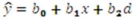 ,a dummy variable d affects the slope of the line.
,a dummy variable d affects the slope of the line. Question
Question
Question
Question
Consider the model y = β0 + β1x + β2d + ε,where x is a quantitative variable and d is a dummy variable.We can use sample data to estimate the model as:
A) = b0 + b1x + b2d
B) = b0 + b1x
C) = b0 + b2d
D)
A)
= b0 + b1x + b2dB)
= b0 + b1xC)
= b0 + b2dD)
Question
Question
Question
Question
Question
Question
Question
Question
For the linear probability model y = β0 + β1x + ε,the predictions made by  can be always interpreted as probabilities.
can be always interpreted as probabilities. Question
Exhibit 17.2.To examine the differences between salaries of male and female middle managers of a large bank,90 individuals were randomly selected and the following variables considered: Salary = the monthly salary (excluding fringe benefits and bonuses),
Educ = the number of years of education,
Exper = the number of months of experience,
Train = the number of weeks of training,
Gender = the gender of an individual;1 for males,and 0 for females.
Also,the following Excel partial outputs corresponding to the following models are available:
Model A: Salary = β0 + β1Educ + β2Exper + β3Train + β4Gender + ε Model B: Salary = β0 + β1Educ + β2Exper + β3Gender + ε
  Refer to Exhibit 17.2.Using Model B,what is the regression equation found by Excel for females?
A) = 4713.2506 + 139.5366Educ + 3.3488Exper + 609.2505Gender
B) = 5322.5011 + 139.5366Educ + 3.3488Expe
C) = 4713.2506 + 139.5366Educ + 3.3488Expe
D)
Educ = the number of years of education,
Exper = the number of months of experience,
Train = the number of weeks of training,
Gender = the gender of an individual;1 for males,and 0 for females.
Also,the following Excel partial outputs corresponding to the following models are available:
Model A: Salary = β0 + β1Educ + β2Exper + β3Train + β4Gender + ε
Model B: Salary = β0 + β1Educ + β2Exper + β3Gender + ε Refer to Exhibit 17.2.Using Model B,what is the regression equation found by Excel for females?A)
= 4713.2506 + 139.5366Educ + 3.3488Exper + 609.2505GenderB)
= 5322.5011 + 139.5366Educ + 3.3488ExpeC)
= 4713.2506 + 139.5366Educ + 3.3488ExpeD)
Question
Exhibit 17.2.To examine the differences between salaries of male and female middle managers of a large bank,90 individuals were randomly selected and the following variables considered: Salary = the monthly salary (excluding fringe benefits and bonuses),
Educ = the number of years of education,
Exper = the number of months of experience,
Train = the number of weeks of training,
Gender = the gender of an individual;1 for males,and 0 for females.
Also,the following Excel partial outputs corresponding to the following models are available:
Model A: Salary = β0 + β1Educ + β2Exper + β3Train + β4Gender + ε Model B: Salary = β0 + β1Educ + β2Exper + β3Gender + ε
  Refer to Exhibit 17.2.Using Model B,what is the regression equation found by Excel for males?
A) = 4713.2506 + 139.5366Educ + 3.3488Exper + 609.2505Gender
B) = 5322.5011 + 139.5366Educ + 3.3488Expe
C) = 4713.2506 + 139.5366Educ + 3.3488Expe
D)
Educ = the number of years of education,
Exper = the number of months of experience,
Train = the number of weeks of training,
Gender = the gender of an individual;1 for males,and 0 for females.
Also,the following Excel partial outputs corresponding to the following models are available:
Model A: Salary = β0 + β1Educ + β2Exper + β3Train + β4Gender + ε
Model B: Salary = β0 + β1Educ + β2Exper + β3Gender + ε Refer to Exhibit 17.2.Using Model B,what is the regression equation found by Excel for males?A)
= 4713.2506 + 139.5366Educ + 3.3488Exper + 609.2505GenderB)
= 5322.5011 + 139.5366Educ + 3.3488ExpeC)
= 4713.2506 + 139.5366Educ + 3.3488ExpeD)
Question
Question
Exhibit 17.2.To examine the differences between salaries of male and female middle managers of a large bank,90 individuals were randomly selected and the following variables considered: Salary = the monthly salary (excluding fringe benefits and bonuses),
Educ = the number of years of education,
Exper = the number of months of experience,
Train = the number of weeks of training,
Gender = the gender of an individual;1 for males,and 0 for females.
Also,the following Excel partial outputs corresponding to the following models are available:
Model A: Salary = β0 + β1Educ + β2Exper + β3Train + β4Gender + ε Model B: Salary = β0 + β1Educ + β2Exper + β3Gender + ε
  Refer to Exhibit 17.2.Using Model A,what is the estimated average difference between the salaries of male and female employees with the same years of education,months of experience,and weeks of training?
A)About $(4663 + 141 + 3 + 1 + 615)= $5423
B)About $(3 + 1 + 615)= $619
C)About $(4663 + 615)= $5278
D)About $615
Educ = the number of years of education,
Exper = the number of months of experience,
Train = the number of weeks of training,
Gender = the gender of an individual;1 for males,and 0 for females.
Also,the following Excel partial outputs corresponding to the following models are available:
Model A: Salary = β0 + β1Educ + β2Exper + β3Train + β4Gender + ε
Model B: Salary = β0 + β1Educ + β2Exper + β3Gender + ε Refer to Exhibit 17.2.Using Model A,what is the estimated average difference between the salaries of male and female employees with the same years of education,months of experience,and weeks of training?A)About $(4663 + 141 + 3 + 1 + 615)= $5423
B)About $(3 + 1 + 615)= $619
C)About $(4663 + 615)= $5278
D)About $615
Question
Exhibit 17.1.A researcher has developed the following regression equation to predict the prices of luxurious Oceanside condominium units,  , where
Price = the price of a unit (in $thousands),
Size = the square footage (in square feet),
View = a dummy variable taking on 1 for an ocean view unit,and 0 for a bay view unit.
Refer to Exhibit 17.1.What is the predicted price of an ocean view unit with 1500 square feet?
A)$315,000
B)$3,150,000
C)$265,000
D)$275,000
, wherePrice = the price of a unit (in $thousands),
Size = the square footage (in square feet),
View = a dummy variable taking on 1 for an ocean view unit,and 0 for a bay view unit.
Refer to Exhibit 17.1.What is the predicted price of an ocean view unit with 1500 square feet?
A)$315,000
B)$3,150,000
C)$265,000
D)$275,000
Question
Exhibit 17.2.To examine the differences between salaries of male and female middle managers of a large bank,90 individuals were randomly selected and the following variables considered: Salary = the monthly salary (excluding fringe benefits and bonuses),
Educ = the number of years of education,
Exper = the number of months of experience,
Train = the number of weeks of training,
Gender = the gender of an individual;1 for males,and 0 for females.
Also,the following Excel partial outputs corresponding to the following models are available:
Model A: Salary = β0 + β1Educ + β2Exper + β3Train + β4Gender + ε Model B: Salary = β0 + β1Educ + β2Exper + β3Gender + ε
  Refer to Exhibit 17.2.Under the assumption of the same years of education and months of experience,what is the p-value for testing whether the mean salary of males is greater than the mean salary of females using Model B?
A)At least 0.025
B)Less than 0.025 but at least 0.01
C)Less than 0.01 but at least 0.005
D)Less than 0.005
Educ = the number of years of education,
Exper = the number of months of experience,
Train = the number of weeks of training,
Gender = the gender of an individual;1 for males,and 0 for females.
Also,the following Excel partial outputs corresponding to the following models are available:
Model A: Salary = β0 + β1Educ + β2Exper + β3Train + β4Gender + ε
Model B: Salary = β0 + β1Educ + β2Exper + β3Gender + ε Refer to Exhibit 17.2.Under the assumption of the same years of education and months of experience,what is the p-value for testing whether the mean salary of males is greater than the mean salary of females using Model B?A)At least 0.025
B)Less than 0.025 but at least 0.01
C)Less than 0.01 but at least 0.005
D)Less than 0.005
Question
Consider the model y = β0 + β1x + β2d + ε,where x is a quantitative variable and d is a dummy variable.For d = 1,the predicted value of y is computed as:
A) = b0 + b1x + b2x
B) = b0 + b1x
C) = (b0 + b1)x + b2
D)
A)
= b0 + b1x + b2xB)
= b0 + b1xC)
= (b0 + b1)x + b2D)
Question
Exhibit 17.2.To examine the differences between salaries of male and female middle managers of a large bank,90 individuals were randomly selected and the following variables considered: Salary = the monthly salary (excluding fringe benefits and bonuses),
Educ = the number of years of education,
Exper = the number of months of experience,
Train = the number of weeks of training,
Gender = the gender of an individual;1 for males,and 0 for females.
Also,the following Excel partial outputs corresponding to the following models are available:
Model A: Salary = β0 + β1Educ + β2Exper + β3Train + β4Gender + ε Model B: Salary = β0 + β1Educ + β2Exper + β3Gender + ε
  Refer to Exhibit 17.2.What is the regression equation found by Excel for Model A?
A) = 4663.31 + 140.66Educ + 3.36Exper + 1.17Train + 615.15Gende
B) = 365.37 + 20.16Educ + 0.47Exper + 3.72Train + 97.33Gender
C) = 12.76 + 6.98Educ + 7.15Exper + 0.31Rrain + 6.32Gender
D)
Educ = the number of years of education,
Exper = the number of months of experience,
Train = the number of weeks of training,
Gender = the gender of an individual;1 for males,and 0 for females.
Also,the following Excel partial outputs corresponding to the following models are available:
Model A: Salary = β0 + β1Educ + β2Exper + β3Train + β4Gender + ε
Model B: Salary = β0 + β1Educ + β2Exper + β3Gender + ε Refer to Exhibit 17.2.What is the regression equation found by Excel for Model A?A)
= 4663.31 + 140.66Educ + 3.36Exper + 1.17Train + 615.15GendeB)
= 365.37 + 20.16Educ + 0.47Exper + 3.72Train + 97.33GenderC)
= 12.76 + 6.98Educ + 7.15Exper + 0.31Rrain + 6.32GenderD)
Question
Question
Question
Exhibit 17.2.To examine the differences between salaries of male and female middle managers of a large bank,90 individuals were randomly selected and the following variables considered: Salary = the monthly salary (excluding fringe benefits and bonuses),
Educ = the number of years of education,
Exper = the number of months of experience,
Train = the number of weeks of training,
Gender = the gender of an individual;1 for males,and 0 for females.
Also,the following Excel partial outputs corresponding to the following models are available:
Model A: Salary = β0 + β1Educ + β2Exper + β3Train + β4Gender + ε Model B: Salary = β0 + β1Educ + β2Exper + β3Gender + ε
  Refer to Exhibit 17.2.Which of the explanatory variables in Model A is most likely to be tested for the individual significance?
A)Educ
B)Exper
C)Train
D)Gender
Educ = the number of years of education,
Exper = the number of months of experience,
Train = the number of weeks of training,
Gender = the gender of an individual;1 for males,and 0 for females.
Also,the following Excel partial outputs corresponding to the following models are available:
Model A: Salary = β0 + β1Educ + β2Exper + β3Train + β4Gender + ε
Model B: Salary = β0 + β1Educ + β2Exper + β3Gender + ε Refer to Exhibit 17.2.Which of the explanatory variables in Model A is most likely to be tested for the individual significance?A)Educ
B)Exper
C)Train
D)Gender
Question
Exhibit 17.2.To examine the differences between salaries of male and female middle managers of a large bank,90 individuals were randomly selected and the following variables considered: Salary = the monthly salary (excluding fringe benefits and bonuses),
Educ = the number of years of education,
Exper = the number of months of experience,
Train = the number of weeks of training,
Gender = the gender of an individual;1 for males,and 0 for females.
Also,the following Excel partial outputs corresponding to the following models are available:
Model A: Salary = β0 + β1Educ + β2Exper + β3Train + β4Gender + ε Model B: Salary = β0 + β1Educ + β2Exper + β3Gender + ε
  Refer to Exhibit 17.2.A group of female managers considers a discrimination lawsuit if on average their salaries could be statistically proven to be lower by more than $500 than the salaries of their male peers with the same level of education and experience.Using Model B,what is the conclusion of the appropriate test at 10% significance level?
A)Do not reject H0;the salaries of female managers cannot be proven to be lower on average by more than $500.
B)Reject H0;the salaries of female managers cannot be proven to be lower on average by more than $500.
C)Do not reject H0;the salaries of female mangers are lower on average by more than $500.
D)Reject H0;the salaries of female mangers are lower on average by more than $500.
Educ = the number of years of education,
Exper = the number of months of experience,
Train = the number of weeks of training,
Gender = the gender of an individual;1 for males,and 0 for females.
Also,the following Excel partial outputs corresponding to the following models are available:
Model A: Salary = β0 + β1Educ + β2Exper + β3Train + β4Gender + ε
Model B: Salary = β0 + β1Educ + β2Exper + β3Gender + ε Refer to Exhibit 17.2.A group of female managers considers a discrimination lawsuit if on average their salaries could be statistically proven to be lower by more than $500 than the salaries of their male peers with the same level of education and experience.Using Model B,what is the conclusion of the appropriate test at 10% significance level?A)Do not reject H0;the salaries of female managers cannot be proven to be lower on average by more than $500.
B)Reject H0;the salaries of female managers cannot be proven to be lower on average by more than $500.
C)Do not reject H0;the salaries of female mangers are lower on average by more than $500.
D)Reject H0;the salaries of female mangers are lower on average by more than $500.
Question
Exhibit 17.1.A researcher has developed the following regression equation to predict the prices of luxurious Oceanside condominium units,  , where
Price = the price of a unit (in $thousands),
Size = the square footage (in square feet),
View = a dummy variable taking on 1 for an ocean view unit,and 0 for a bay view unit.
Refer to Exhibit 17.1.What is the predicted price of a bay view unit measuring 1500 square feet?
A)$315,000
B)$2,650,000
C)$265,000
D)$225,000
, wherePrice = the price of a unit (in $thousands),
Size = the square footage (in square feet),
View = a dummy variable taking on 1 for an ocean view unit,and 0 for a bay view unit.
Refer to Exhibit 17.1.What is the predicted price of a bay view unit measuring 1500 square feet?
A)$315,000
B)$2,650,000
C)$265,000
D)$225,000
Question
Question
Exhibit 17.2.To examine the differences between salaries of male and female middle managers of a large bank,90 individuals were randomly selected and the following variables considered: Salary = the monthly salary (excluding fringe benefits and bonuses),
Educ = the number of years of education,
Exper = the number of months of experience,
Train = the number of weeks of training,
Gender = the gender of an individual;1 for males,and 0 for females.
Also,the following Excel partial outputs corresponding to the following models are available:
Model A: Salary = β0 + β1Educ + β2Exper + β3Train + β4Gender + ε Model B: Salary = β0 + β1Educ + β2Exper + β3Gender + ε
  Refer to Exhibit 17.2.When testing the individual significance of Train in Model A,what is the test conclusion at 10% significance level?
A)Do not reject H0;Train is significant
B)Reject H0;Train is significant
C)Reject H0;Train does not seem to be significant
D)Do not reject H0;Train does not seem to be significant
Educ = the number of years of education,
Exper = the number of months of experience,
Train = the number of weeks of training,
Gender = the gender of an individual;1 for males,and 0 for females.
Also,the following Excel partial outputs corresponding to the following models are available:
Model A: Salary = β0 + β1Educ + β2Exper + β3Train + β4Gender + ε
Model B: Salary = β0 + β1Educ + β2Exper + β3Gender + ε Refer to Exhibit 17.2.When testing the individual significance of Train in Model A,what is the test conclusion at 10% significance level?A)Do not reject H0;Train is significant
B)Reject H0;Train is significant
C)Reject H0;Train does not seem to be significant
D)Do not reject H0;Train does not seem to be significant
Question
Exhibit 17.3.Consider the regression model, Humidity = β0 + β1Temperature + β2Spring + β3Summer + β4Fall + β5Rain + ε,
Where the dummy variables Spring,Summer,and Fall represent the qualitative variable Season (spring,summer,fall,winter),and the dummy variable Rain is defined as Rain = 1 if rainy day,Rain = 0 otherwise.
Refer to Exhibit 17.3.What is the regression equation for the summer days?
A) = (b0 + b3)+ b1Temperature + b5Rain
B) = b0 + b1Temperature + b5Rain
C) = b0 + b1Temperature + b2Spring + b5Rain
D)
Where the dummy variables Spring,Summer,and Fall represent the qualitative variable Season (spring,summer,fall,winter),and the dummy variable Rain is defined as Rain = 1 if rainy day,Rain = 0 otherwise.
Refer to Exhibit 17.3.What is the regression equation for the summer days?
A)
= (b0 + b3)+ b1Temperature + b5RainB)
= b0 + b1Temperature + b5RainC)
= b0 + b1Temperature + b2Spring + b5RainD)
Question
Exhibit 17.1.A researcher has developed the following regression equation to predict the prices of luxurious Oceanside condominium units,  , where
Price = the price of a unit (in $thousands),
Size = the square footage (in square feet),
View = a dummy variable taking on 1 for an ocean view unit,and 0 for a bay view unit.
Refer to Exhibit 17.1.What is the predicted difference in prices of the ocean view and bay view units with the same square footage?
A)$40,000
B)$90,000
C)$500,000
D)$50,000
, wherePrice = the price of a unit (in $thousands),
Size = the square footage (in square feet),
View = a dummy variable taking on 1 for an ocean view unit,and 0 for a bay view unit.
Refer to Exhibit 17.1.What is the predicted difference in prices of the ocean view and bay view units with the same square footage?
A)$40,000
B)$90,000
C)$500,000
D)$50,000
Question
Exhibit 17.2.To examine the differences between salaries of male and female middle managers of a large bank,90 individuals were randomly selected and the following variables considered: Salary = the monthly salary (excluding fringe benefits and bonuses),
Educ = the number of years of education,
Exper = the number of months of experience,
Train = the number of weeks of training,
Gender = the gender of an individual;1 for males,and 0 for females.
Also,the following Excel partial outputs corresponding to the following models are available:
Model A: Salary = β0 + β1Educ + β2Exper + β3Train + β4Gender + ε Model B: Salary = β0 + β1Educ + β2Exper + β3Gender + ε
  Refer to Exhibit 17.2.Under the assumption of the same years of education and months of experience,what is the null hypothesis for testing whether the mean salary of males is greater than the mean salary of females using Model B?
A)H0: β3 ≤ 0
B)H0: β3 ≥ 0
C)H0: β3 > 0
D)H0: β3 = 0
Educ = the number of years of education,
Exper = the number of months of experience,
Train = the number of weeks of training,
Gender = the gender of an individual;1 for males,and 0 for females.
Also,the following Excel partial outputs corresponding to the following models are available:
Model A: Salary = β0 + β1Educ + β2Exper + β3Train + β4Gender + ε
Model B: Salary = β0 + β1Educ + β2Exper + β3Gender + ε Refer to Exhibit 17.2.Under the assumption of the same years of education and months of experience,what is the null hypothesis for testing whether the mean salary of males is greater than the mean salary of females using Model B?A)H0: β3 ≤ 0
B)H0: β3 ≥ 0
C)H0: β3 > 0
D)H0: β3 = 0
Question
Exhibit 17.2.To examine the differences between salaries of male and female middle managers of a large bank,90 individuals were randomly selected and the following variables considered: Salary = the monthly salary (excluding fringe benefits and bonuses),
Educ = the number of years of education,
Exper = the number of months of experience,
Train = the number of weeks of training,
Gender = the gender of an individual;1 for males,and 0 for females.
Also,the following Excel partial outputs corresponding to the following models are available:
Model A: Salary = β0 + β1Educ + β2Exper + β3Train + β4Gender + ε Model B: Salary = β0 + β1Educ + β2Exper + β3Gender + ε
  Refer to Exhibit 17.2.A group of female managers considers a discrimination lawsuit if on average their salaries can be statistically proven to be lower by more than $500 than the salaries of their male peers with the same level of education and experience.Using Model B,what is the alternative hypothesis for testing the lawsuit condition?
A)HA: β3 ≤ 500
B)HA: β3 < 500
C)HA: β3 ≠ 500
D)HA: β3 > 500
Educ = the number of years of education,
Exper = the number of months of experience,
Train = the number of weeks of training,
Gender = the gender of an individual;1 for males,and 0 for females.
Also,the following Excel partial outputs corresponding to the following models are available:
Model A: Salary = β0 + β1Educ + β2Exper + β3Train + β4Gender + ε
Model B: Salary = β0 + β1Educ + β2Exper + β3Gender + ε Refer to Exhibit 17.2.A group of female managers considers a discrimination lawsuit if on average their salaries can be statistically proven to be lower by more than $500 than the salaries of their male peers with the same level of education and experience.Using Model B,what is the alternative hypothesis for testing the lawsuit condition?A)HA: β3 ≤ 500
B)HA: β3 < 500
C)HA: β3 ≠ 500
D)HA: β3 > 500
Question
Consider the regression equation  = b0 + b1x + b2d with a dummy variable d.If d increases from 0 to 1,the change in the intercept is given by:
A)b0
B)b0 + b1
C)b2
D)b0 + b2
= b0 + b1x + b2d with a dummy variable d.If d increases from 0 to 1,the change in the intercept is given by:A)b0
B)b0 + b1
C)b2
D)b0 + b2
Question
Exhibit 17.3.Consider the regression model, Humidity = β0 + β1Temperature + β2Spring + β3Summer + β4Fall + β5Rain + ε,
Where the dummy variables Spring,Summer,and Fall represent the qualitative variable Season (spring,summer,fall,winter),and the dummy variable Rain is defined as Rain = 1 if rainy day,Rain = 0 otherwise.
Refer to Exhibit 17.3.What is the regression equation for the summer rainy days?
A) = (b0 + b3)+ b1Temperature
B) = (b0 + b5)+ b1Temperature
C) = b0 + b1Temperature + b2Spring + b4Fall
D)
Where the dummy variables Spring,Summer,and Fall represent the qualitative variable Season (spring,summer,fall,winter),and the dummy variable Rain is defined as Rain = 1 if rainy day,Rain = 0 otherwise.
Refer to Exhibit 17.3.What is the regression equation for the summer rainy days?
A)
= (b0 + b3)+ b1TemperatureB)
= (b0 + b5)+ b1TemperatureC)
= b0 + b1Temperature + b2Spring + b4FallD)
Question
In the model y = β0 + β1x + β2d + β3xd + ε,for a given x and d = 1,the predicted value of y is given by:
A) = b0 + b1x + b2 + b3x
B) = b0 + b2 + b1x + b3x
C) = (b0 + b2)+ (b1 + b3)x
D)All of the above
A)
= b0 + b1x + b2 + b3xB)
= b0 + b2 + b1x + b3xC)
= (b0 + b2)+ (b1 + b3)xD)All of the above
Question
Question
In the regression equation  = b0 + b1x + b2dx with a dummy variable d,when d changes from 0 to 1,the change in the slope of the corresponding lines is given by:
A)b0
B)b0 + b1
C)b2
D)b0 + b2
= b0 + b1x + b2dx with a dummy variable d,when d changes from 0 to 1,the change in the slope of the corresponding lines is given by:A)b0
B)b0 + b1
C)b2
D)b0 + b2
Question
Exhibit 17.4.A researcher wants to examine how the remaining balance on $100,000 loans taken 10-20 years ago depends on whether the loan was a prime or sub-prime loan.He collected a sample of 25 prime loans and 25 sub-prime loans and records the data in the following variables: Balance = the remaining amount of loan to be paid off (in dollars),
Time = the time elapsed from taking the loan,
Prime = a dummy variable assuming 1 for prime loans,and 0 for sub-prime loans.
The regression results obtained for the models:
Model A: Balance = β0 + β1Prime + ε
Model B: Balance = β0 + β1Time + β2Prime + β3Time × Prime + ε
Model C: Balance = β0 + β1Prime + β2Time × Prime + ε,
Are summarized below.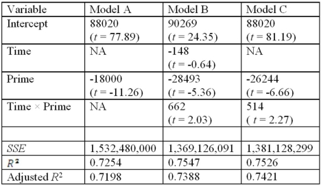 Note.The values of relevant test statistics are shown in parentheses below the estimated coefficients.
Refer to Exhibit 17.4.What is the p-value for testing the significance of Time in Model B?
A)Less than 0.10
B)Less than 0.20 but at least 0.10
C)Less than 0.40 but at least 0.20
D)More than 0.40
Time = the time elapsed from taking the loan,
Prime = a dummy variable assuming 1 for prime loans,and 0 for sub-prime loans.
The regression results obtained for the models:
Model A: Balance = β0 + β1Prime + ε
Model B: Balance = β0 + β1Time + β2Prime + β3Time × Prime + ε
Model C: Balance = β0 + β1Prime + β2Time × Prime + ε,
Are summarized below.
Note.The values of relevant test statistics are shown in parentheses below the estimated coefficients.Refer to Exhibit 17.4.What is the p-value for testing the significance of Time in Model B?
A)Less than 0.10
B)Less than 0.20 but at least 0.10
C)Less than 0.40 but at least 0.20
D)More than 0.40
Question
Exhibit 17.4.A researcher wants to examine how the remaining balance on $100,000 loans taken 10-20 years ago depends on whether the loan was a prime or sub-prime loan.He collected a sample of 25 prime loans and 25 sub-prime loans and records the data in the following variables: Balance = the remaining amount of loan to be paid off (in dollars),
Time = the time elapsed from taking the loan,
Prime = a dummy variable assuming 1 for prime loans,and 0 for sub-prime loans.
The regression results obtained for the models:
Model A: Balance = β0 + β1Prime + ε
Model B: Balance = β0 + β1Time + β2Prime + β3Time × Prime + ε
Model C: Balance = β0 + β1Prime + β2Time × Prime + ε,
Are summarized below. Note.The values of relevant test statistics are shown in parentheses below the estimated coefficients.
Refer to Exhibit 17.4.Which of the three models would you choose to make the predictions of the remaining loan balance?
A)Model A
B)Model B
C)Model C
D)Any model
Time = the time elapsed from taking the loan,
Prime = a dummy variable assuming 1 for prime loans,and 0 for sub-prime loans.
The regression results obtained for the models:
Model A: Balance = β0 + β1Prime + ε
Model B: Balance = β0 + β1Time + β2Prime + β3Time × Prime + ε
Model C: Balance = β0 + β1Prime + β2Time × Prime + ε,
Are summarized below.
Note.The values of relevant test statistics are shown in parentheses below the estimated coefficients.Refer to Exhibit 17.4.Which of the three models would you choose to make the predictions of the remaining loan balance?
A)Model A
B)Model B
C)Model C
D)Any model
Question
Question
Question
Exhibit 17.4.A researcher wants to examine how the remaining balance on $100,000 loans taken 10-20 years ago depends on whether the loan was a prime or sub-prime loan.He collected a sample of 25 prime loans and 25 sub-prime loans and records the data in the following variables: Balance = the remaining amount of loan to be paid off (in dollars),
Time = the time elapsed from taking the loan,
Prime = a dummy variable assuming 1 for prime loans,and 0 for sub-prime loans.
The regression results obtained for the models:
Model A: Balance = β0 + β1Prime + ε
Model B: Balance = β0 + β1Time + β2Prime + β3Time × Prime + ε
Model C: Balance = β0 + β1Prime + β2Time × Prime + ε,
Are summarized below. Note.The values of relevant test statistics are shown in parentheses below the estimated coefficients.
Refer to Exhibit 17.4.Using Model B,what is the value of the test statistic for testing the joint significance of the variable Time and the interaction variable Time × Prime?
A)-0.64
B)-5.36
C)2.03
D)2.74
Time = the time elapsed from taking the loan,
Prime = a dummy variable assuming 1 for prime loans,and 0 for sub-prime loans.
The regression results obtained for the models:
Model A: Balance = β0 + β1Prime + ε
Model B: Balance = β0 + β1Time + β2Prime + β3Time × Prime + ε
Model C: Balance = β0 + β1Prime + β2Time × Prime + ε,
Are summarized below.
Note.The values of relevant test statistics are shown in parentheses below the estimated coefficients.Refer to Exhibit 17.4.Using Model B,what is the value of the test statistic for testing the joint significance of the variable Time and the interaction variable Time × Prime?
A)-0.64
B)-5.36
C)2.03
D)2.74
Question
Exhibit 17.3.Consider the regression model, Humidity = β0 + β1Temperature + β2Spring + β3Summer + β4Fall + β5Rain + ε,
Where the dummy variables Spring,Summer,and Fall represent the qualitative variable Season (spring,summer,fall,winter),and the dummy variable Rain is defined as Rain = 1 if rainy day,Rain = 0 otherwise.
Refer to Exhibit 17.3.What is the regression equation for the winter rainy days?
A) = (b0 + b3)+ b1Temperature + b5Rain
B) = (b0 + b5)+ b1Temperature
C) = (b0 + b2 + b3 + b4 + b5)+ b1Temperature
D)
Where the dummy variables Spring,Summer,and Fall represent the qualitative variable Season (spring,summer,fall,winter),and the dummy variable Rain is defined as Rain = 1 if rainy day,Rain = 0 otherwise.
Refer to Exhibit 17.3.What is the regression equation for the winter rainy days?
A)
= (b0 + b3)+ b1Temperature + b5RainB)
= (b0 + b5)+ b1TemperatureC)
= (b0 + b2 + b3 + b4 + b5)+ b1TemperatureD)
Question
Question
Question
Question
Question
Exhibit 17.3.Consider the regression model, Humidity = β0 + β1Temperature + β2Spring + β3Summer + β4Fall + β5Rain + ε,
Where the dummy variables Spring,Summer,and Fall represent the qualitative variable Season (spring,summer,fall,winter),and the dummy variable Rain is defined as Rain = 1 if rainy day,Rain = 0 otherwise.
Refer to Exhibit 17.3.What is the regression equation for the winter days?
A) = (b0 + b3)+ b1Temperature + b5Rain
B) = (b0 + b2 + b3 + b4)+ b1Temperature + b5Rain
C) = b0 + b1Temperature + b5Rain
D)
Where the dummy variables Spring,Summer,and Fall represent the qualitative variable Season (spring,summer,fall,winter),and the dummy variable Rain is defined as Rain = 1 if rainy day,Rain = 0 otherwise.
Refer to Exhibit 17.3.What is the regression equation for the winter days?
A)
= (b0 + b3)+ b1Temperature + b5RainB)
= (b0 + b2 + b3 + b4)+ b1Temperature + b5RainC)
= b0 + b1Temperature + b5RainD)
Question
Exhibit 17.4.A researcher wants to examine how the remaining balance on $100,000 loans taken 10-20 years ago depends on whether the loan was a prime or sub-prime loan.He collected a sample of 25 prime loans and 25 sub-prime loans and records the data in the following variables: Balance = the remaining amount of loan to be paid off (in dollars),
Time = the time elapsed from taking the loan,
Prime = a dummy variable assuming 1 for prime loans,and 0 for sub-prime loans.
The regression results obtained for the models:
Model A: Balance = β0 + β1Prime + ε
Model B: Balance = β0 + β1Time + β2Prime + β3Time × Prime + ε
Model C: Balance = β0 + β1Prime + β2Time × Prime + ε,
Are summarized below. Note.The values of relevant test statistics are shown in parentheses below the estimated coefficients.
Refer to Exhibit 17.4.Using Model C,what is the predicted balance on a $100,000 prime loan taken 15 years ago?
A)$88,020
B)$69,486
C)$74,591
D)$82,183
Time = the time elapsed from taking the loan,
Prime = a dummy variable assuming 1 for prime loans,and 0 for sub-prime loans.
The regression results obtained for the models:
Model A: Balance = β0 + β1Prime + ε
Model B: Balance = β0 + β1Time + β2Prime + β3Time × Prime + ε
Model C: Balance = β0 + β1Prime + β2Time × Prime + ε,
Are summarized below.
Note.The values of relevant test statistics are shown in parentheses below the estimated coefficients.Refer to Exhibit 17.4.Using Model C,what is the predicted balance on a $100,000 prime loan taken 15 years ago?
A)$88,020
B)$69,486
C)$74,591
D)$82,183
Question
Exhibit 17.4.A researcher wants to examine how the remaining balance on $100,000 loans taken 10-20 years ago depends on whether the loan was a prime or sub-prime loan.He collected a sample of 25 prime loans and 25 sub-prime loans and records the data in the following variables: Balance = the remaining amount of loan to be paid off (in dollars),
Time = the time elapsed from taking the loan,
Prime = a dummy variable assuming 1 for prime loans,and 0 for sub-prime loans.
The regression results obtained for the models:
Model A: Balance = β0 + β1Prime + ε
Model B: Balance = β0 + β1Time + β2Prime + β3Time × Prime + ε
Model C: Balance = β0 + β1Prime + β2Time × Prime + ε,
Are summarized below. Note.The values of relevant test statistics are shown in parentheses below the estimated coefficients.
Refer to Exhibit 17.4.Using Model B,what is the null hypothesis for testing the joint significance of the variable Time and the interaction variable Time × Prime?
A)H0: β1 = β2 = β3 = 0
B)H0: β1 = 0 and β3 = 0
C)H0: β1 = 0 or β3 = 0
D)H0: β1 ≠ 0 or β3 ≠ 0
Time = the time elapsed from taking the loan,
Prime = a dummy variable assuming 1 for prime loans,and 0 for sub-prime loans.
The regression results obtained for the models:
Model A: Balance = β0 + β1Prime + ε
Model B: Balance = β0 + β1Time + β2Prime + β3Time × Prime + ε
Model C: Balance = β0 + β1Prime + β2Time × Prime + ε,
Are summarized below.
Note.The values of relevant test statistics are shown in parentheses below the estimated coefficients.Refer to Exhibit 17.4.Using Model B,what is the null hypothesis for testing the joint significance of the variable Time and the interaction variable Time × Prime?
A)H0: β1 = β2 = β3 = 0
B)H0: β1 = 0 and β3 = 0
C)H0: β1 = 0 or β3 = 0
D)H0: β1 ≠ 0 or β3 ≠ 0
Question
Consider the regression equation  = b0 + b1xd with b1 > 0 and a dummy variable d.If d changes from 0 to 1,which of the following is true?
A)The intercept increases by b0 + b1.
B)The intercept increases by b1.
C)The slope increases by b0 + b1.
D)The slope increases by b1.
= b0 + b1xd with b1 > 0 and a dummy variable d.If d changes from 0 to 1,which of the following is true?A)The intercept increases by b0 + b1.
B)The intercept increases by b1.
C)The slope increases by b0 + b1.
D)The slope increases by b1.
Question
Question
Exhibit 17.4.A researcher wants to examine how the remaining balance on $100,000 loans taken 10-20 years ago depends on whether the loan was a prime or sub-prime loan.He collected a sample of 25 prime loans and 25 sub-prime loans and records the data in the following variables: Balance = the remaining amount of loan to be paid off (in dollars),
Time = the time elapsed from taking the loan,
Prime = a dummy variable assuming 1 for prime loans,and 0 for sub-prime loans.
The regression results obtained for the models:
Model A: Balance = β0 + β1Prime + ε
Model B: Balance = β0 + β1Time + β2Prime + β3Time × Prime + ε
Model C: Balance = β0 + β1Prime + β2Time × Prime + ε,
Are summarized below. Note.The values of relevant test statistics are shown in parentheses below the estimated coefficients.
Refer to Exhibit 17.4.Using Model B,what is the alternative hypothesis for testing the significance of Time?
A)HA: β1 = 0
B)HA: β1 = 0 and β3 = 0
C)HA: β1 ≠ 0
D)HA: β1 ≠ 0 or β3 ≠ 0
Time = the time elapsed from taking the loan,
Prime = a dummy variable assuming 1 for prime loans,and 0 for sub-prime loans.
The regression results obtained for the models:
Model A: Balance = β0 + β1Prime + ε
Model B: Balance = β0 + β1Time + β2Prime + β3Time × Prime + ε
Model C: Balance = β0 + β1Prime + β2Time × Prime + ε,
Are summarized below.
Note.The values of relevant test statistics are shown in parentheses below the estimated coefficients.Refer to Exhibit 17.4.Using Model B,what is the alternative hypothesis for testing the significance of Time?
A)HA: β1 = 0
B)HA: β1 = 0 and β3 = 0
C)HA: β1 ≠ 0
D)HA: β1 ≠ 0 or β3 ≠ 0

Unlock Deck
Sign up to unlock the cards in this deck!
Unlock Deck
Unlock Deck
1/117
Play
Full screen (f)
Deck 17: Regression Models With Dummy Variables
1
Exhibit 17.8.A realtor wants to predict and compare the prices of homes in three neighboring locations.She considers the following linear models:
Model A: Price = β0 + β1Size + β2Age + ε,
Model B: Price = β0 + β1Size + β2Loc1 + β3Loc2 + ε,
Model C: Price = β0 + β1Size + β2Age + β3Loc1 + β4Loc2 + ε,
where,
Price = the price of a home (in $thousands),
Size = the square footage (in square feet),
Loc1 = a dummy variable taking on 1 for Location 1,and 0 otherwise,
Loc2 = a dummy variable taking on 1 for Location 2,and 0 otherwise.
After collecting data on 52 sales and applying regression,her findings were summarized in the following table.
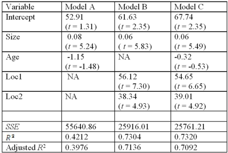 Note: The values of relevant test statistics are shown in parentheses below the estimated coefficients.
Refer to Exhibit 17.8.Which of the three models would you choose to make the predictions of the home prices?
2
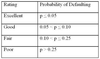
Exhibit 17.9.A bank manager is interested in assigning a rating to the holders of credit cards issued by her bank.The rating is based on the probability of defaulting on credit cards and is as follows.
 To estimate this probability,she decided to use the logistic model:
 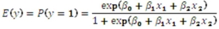 ,
,where,
y = a binary response variable with value 1 corresponding to a default,and 0 to a no default,
x1 = the ratio of the credit card balance to the credit card limit (in percent),
x2 = the ratio of the total debt to the annual income (in percent).
Using Minitab on the sample data,she arrived at the following estimates:
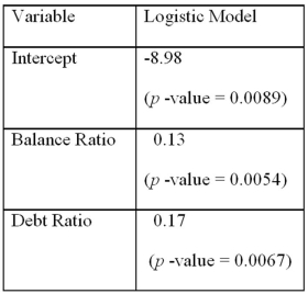 Note: The p-values of the corresponding tests are shown in parentheses below the estimated coefficients.
Refer to Exhibit 17.9.Assuming the debt ratio 30%,compute the increase in the probability of defaulting when the balance ratio goes up from 5% to 15%.
3
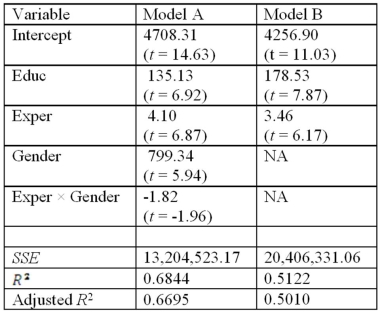
Exhibit 17.7.To examine the differences between salaries of male and female middle managers of a large bank,90 individuals were randomly selected and the following variables considered:
Salary = the monthly salary (excluding fringe benefits and bonuses),
Educ = the number of years of education,
Exper = the number of months of experience,
Gender = the gender of an individual;1 for males,and 0 for females.
The regression results for the models,
Model A: Salary = β0 + β1Educ + β2Exper + β3Gender + β4Exper × Gender + ε,
Model B: Salary = β0 + β1Educ + β2Exper + ε,are summarized below.
 Note.The values of relevant test statistics are shown in parentheses below the estimated coefficients.
Refer to Exhibit 17.7.What is the alternative hypothesis for testing the joint significance of Exper and Exper × Gender in Model A?
4
Exhibit 17.7.To examine the differences between salaries of male and female middle managers of a large bank,90 individuals were randomly selected and the following variables considered:
Salary = the monthly salary (excluding fringe benefits and bonuses),
Educ = the number of years of education,
Exper = the number of months of experience,
Gender = the gender of an individual;1 for males,and 0 for females.
The regression results for the models,
Model A: Salary = β0 + β1Educ + β2Exper + β3Gender + β4Exper × Gender + ε,
Model B: Salary = β0 + β1Educ + β2Exper + ε,are summarized below.
Salary = the monthly salary (excluding fringe benefits and bonuses),
Educ = the number of years of education,
Exper = the number of months of experience,
Gender = the gender of an individual;1 for males,and 0 for females.
The regression results for the models,
Model A: Salary = β0 + β1Educ + β2Exper + β3Gender + β4Exper × Gender + ε,
Model B: Salary = β0 + β1Educ + β2Exper + ε,are summarized below.
Unlock Deck
Unlock for access to all 117 flashcards in this deck.
Unlock Deck
k this deck
5
Exhibit 17.8.A realtor wants to predict and compare the prices of homes in three neighboring locations.She considers the following linear models:
Model A: Price = β0 + β1Size + β2Age + ε,
Model B: Price = β0 + β1Size + β2Loc1 + β3Loc2 + ε,
Model C: Price = β0 + β1Size + β2Age + β3Loc1 + β4Loc2 + ε,
where,
Price = the price of a home (in $thousands),
Size = the square footage (in square feet),
Loc1 = a dummy variable taking on 1 for Location 1,and 0 otherwise,
Loc2 = a dummy variable taking on 1 for Location 2,and 0 otherwise.
After collecting data on 52 sales and applying regression,her findings were summarized in the following table.
Model A: Price = β0 + β1Size + β2Age + ε,
Model B: Price = β0 + β1Size + β2Loc1 + β3Loc2 + ε,
Model C: Price = β0 + β1Size + β2Age + β3Loc1 + β4Loc2 + ε,
where,
Price = the price of a home (in $thousands),
Size = the square footage (in square feet),
Loc1 = a dummy variable taking on 1 for Location 1,and 0 otherwise,
Loc2 = a dummy variable taking on 1 for Location 2,and 0 otherwise.
After collecting data on 52 sales and applying regression,her findings were summarized in the following table.
Unlock Deck
Unlock for access to all 117 flashcards in this deck.
Unlock Deck
k this deck
6
Exhibit 17.8.A realtor wants to predict and compare the prices of homes in three neighboring locations.She considers the following linear models:
Model A: Price = β0 + β1Size + β2Age + ε,
Model B: Price = β0 + β1Size + β2Loc1 + β3Loc2 + ε,
Model C: Price = β0 + β1Size + β2Age + β3Loc1 + β4Loc2 + ε,
where,
Price = the price of a home (in $thousands),
Size = the square footage (in square feet),
Loc1 = a dummy variable taking on 1 for Location 1,and 0 otherwise,
Loc2 = a dummy variable taking on 1 for Location 2,and 0 otherwise.
After collecting data on 52 sales and applying regression,her findings were summarized in the following table.
Model A: Price = β0 + β1Size + β2Age + ε,
Model B: Price = β0 + β1Size + β2Loc1 + β3Loc2 + ε,
Model C: Price = β0 + β1Size + β2Age + β3Loc1 + β4Loc2 + ε,
where,
Price = the price of a home (in $thousands),
Size = the square footage (in square feet),
Loc1 = a dummy variable taking on 1 for Location 1,and 0 otherwise,
Loc2 = a dummy variable taking on 1 for Location 2,and 0 otherwise.
After collecting data on 52 sales and applying regression,her findings were summarized in the following table.
Unlock Deck
Unlock for access to all 117 flashcards in this deck.
Unlock Deck
k this deck
7
Exhibit 17.8.A realtor wants to predict and compare the prices of homes in three neighboring locations.She considers the following linear models:
Model A: Price = β0 + β1Size + β2Age + ε,
Model B: Price = β0 + β1Size + β2Loc1 + β3Loc2 + ε,
Model C: Price = β0 + β1Size + β2Age + β3Loc1 + β4Loc2 + ε,
where,
Price = the price of a home (in $thousands),
Size = the square footage (in square feet),
Loc1 = a dummy variable taking on 1 for Location 1,and 0 otherwise,
Loc2 = a dummy variable taking on 1 for Location 2,and 0 otherwise.
After collecting data on 52 sales and applying regression,her findings were summarized in the following table.
Model A: Price = β0 + β1Size + β2Age + ε,
Model B: Price = β0 + β1Size + β2Loc1 + β3Loc2 + ε,
Model C: Price = β0 + β1Size + β2Age + β3Loc1 + β4Loc2 + ε,
where,
Price = the price of a home (in $thousands),
Size = the square footage (in square feet),
Loc1 = a dummy variable taking on 1 for Location 1,and 0 otherwise,
Loc2 = a dummy variable taking on 1 for Location 2,and 0 otherwise.
After collecting data on 52 sales and applying regression,her findings were summarized in the following table.
Unlock Deck
Unlock for access to all 117 flashcards in this deck.
Unlock Deck
k this deck
8
Exhibit 17.8.A realtor wants to predict and compare the prices of homes in three neighboring locations.She considers the following linear models:
Model A: Price = β0 + β1Size + β2Age + ε,
Model B: Price = β0 + β1Size + β2Loc1 + β3Loc2 + ε,
Model C: Price = β0 + β1Size + β2Age + β3Loc1 + β4Loc2 + ε,
where,
Price = the price of a home (in $thousands),
Size = the square footage (in square feet),
Loc1 = a dummy variable taking on 1 for Location 1,and 0 otherwise,
Loc2 = a dummy variable taking on 1 for Location 2,and 0 otherwise.
After collecting data on 52 sales and applying regression,her findings were summarized in the following table.
Model A: Price = β0 + β1Size + β2Age + ε,
Model B: Price = β0 + β1Size + β2Loc1 + β3Loc2 + ε,
Model C: Price = β0 + β1Size + β2Age + β3Loc1 + β4Loc2 + ε,
where,
Price = the price of a home (in $thousands),
Size = the square footage (in square feet),
Loc1 = a dummy variable taking on 1 for Location 1,and 0 otherwise,
Loc2 = a dummy variable taking on 1 for Location 2,and 0 otherwise.
After collecting data on 52 sales and applying regression,her findings were summarized in the following table.
Unlock Deck
Unlock for access to all 117 flashcards in this deck.
Unlock Deck
k this deck
9
Exhibit 17.9.A bank manager is interested in assigning a rating to the holders of credit cards issued by her bank.The rating is based on the probability of defaulting on credit cards and is as follows.
Unlock Deck
Unlock for access to all 117 flashcards in this deck.
Unlock Deck
k this deck
10
Exhibit 17.8.A realtor wants to predict and compare the prices of homes in three neighboring locations.She considers the following linear models:
Model A: Price = β0 + β1Size + β2Age + ε,
Model B: Price = β0 + β1Size + β2Loc1 + β3Loc2 + ε,
Model C: Price = β0 + β1Size + β2Age + β3Loc1 + β4Loc2 + ε,
where,
Price = the price of a home (in $thousands),
Size = the square footage (in square feet),
Loc1 = a dummy variable taking on 1 for Location 1,and 0 otherwise,
Loc2 = a dummy variable taking on 1 for Location 2,and 0 otherwise.
After collecting data on 52 sales and applying regression,her findings were summarized in the following table.
Model A: Price = β0 + β1Size + β2Age + ε,
Model B: Price = β0 + β1Size + β2Loc1 + β3Loc2 + ε,
Model C: Price = β0 + β1Size + β2Age + β3Loc1 + β4Loc2 + ε,
where,
Price = the price of a home (in $thousands),
Size = the square footage (in square feet),
Loc1 = a dummy variable taking on 1 for Location 1,and 0 otherwise,
Loc2 = a dummy variable taking on 1 for Location 2,and 0 otherwise.
After collecting data on 52 sales and applying regression,her findings were summarized in the following table.
Unlock Deck
Unlock for access to all 117 flashcards in this deck.
Unlock Deck
k this deck
11
Exhibit 17.9.A bank manager is interested in assigning a rating to the holders of credit cards issued by her bank.The rating is based on the probability of defaulting on credit cards and is as follows.
Unlock Deck
Unlock for access to all 117 flashcards in this deck.
Unlock Deck
k this deck
12
Exhibit 17.8.A realtor wants to predict and compare the prices of homes in three neighboring locations.She considers the following linear models:
Model A: Price = β0 + β1Size + β2Age + ε,
Model B: Price = β0 + β1Size + β2Loc1 + β3Loc2 + ε,
Model C: Price = β0 + β1Size + β2Age + β3Loc1 + β4Loc2 + ε,
where,
Price = the price of a home (in $thousands),
Size = the square footage (in square feet),
Loc1 = a dummy variable taking on 1 for Location 1,and 0 otherwise,
Loc2 = a dummy variable taking on 1 for Location 2,and 0 otherwise.
After collecting data on 52 sales and applying regression,her findings were summarized in the following table.
Model A: Price = β0 + β1Size + β2Age + ε,
Model B: Price = β0 + β1Size + β2Loc1 + β3Loc2 + ε,
Model C: Price = β0 + β1Size + β2Age + β3Loc1 + β4Loc2 + ε,
where,
Price = the price of a home (in $thousands),
Size = the square footage (in square feet),
Loc1 = a dummy variable taking on 1 for Location 1,and 0 otherwise,
Loc2 = a dummy variable taking on 1 for Location 2,and 0 otherwise.
After collecting data on 52 sales and applying regression,her findings were summarized in the following table.
Unlock Deck
Unlock for access to all 117 flashcards in this deck.
Unlock Deck
k this deck
13
Exhibit 17.9.A bank manager is interested in assigning a rating to the holders of credit cards issued by her bank.The rating is based on the probability of defaulting on credit cards and is as follows.
Unlock Deck
Unlock for access to all 117 flashcards in this deck.
Unlock Deck
k this deck
14
Exhibit 17.9.A bank manager is interested in assigning a rating to the holders of credit cards issued by her bank.The rating is based on the probability of defaulting on credit cards and is as follows.
Unlock Deck
Unlock for access to all 117 flashcards in this deck.
Unlock Deck
k this deck
15
Exhibit 17.9.A bank manager is interested in assigning a rating to the holders of credit cards issued by her bank.The rating is based on the probability of defaulting on credit cards and is as follows.
Unlock Deck
Unlock for access to all 117 flashcards in this deck.
Unlock Deck
k this deck
16
Exhibit 17.9.A bank manager is interested in assigning a rating to the holders of credit cards issued by her bank.The rating is based on the probability of defaulting on credit cards and is as follows.
Unlock Deck
Unlock for access to all 117 flashcards in this deck.
Unlock Deck
k this deck
17
Exhibit 17.8.A realtor wants to predict and compare the prices of homes in three neighboring locations.She considers the following linear models:
Model A: Price = β0 + β1Size + β2Age + ε,
Model B: Price = β0 + β1Size + β2Loc1 + β3Loc2 + ε,
Model C: Price = β0 + β1Size + β2Age + β3Loc1 + β4Loc2 + ε,
where,
Price = the price of a home (in $thousands),
Size = the square footage (in square feet),
Loc1 = a dummy variable taking on 1 for Location 1,and 0 otherwise,
Loc2 = a dummy variable taking on 1 for Location 2,and 0 otherwise.
After collecting data on 52 sales and applying regression,her findings were summarized in the following table.
Model A: Price = β0 + β1Size + β2Age + ε,
Model B: Price = β0 + β1Size + β2Loc1 + β3Loc2 + ε,
Model C: Price = β0 + β1Size + β2Age + β3Loc1 + β4Loc2 + ε,
where,
Price = the price of a home (in $thousands),
Size = the square footage (in square feet),
Loc1 = a dummy variable taking on 1 for Location 1,and 0 otherwise,
Loc2 = a dummy variable taking on 1 for Location 2,and 0 otherwise.
After collecting data on 52 sales and applying regression,her findings were summarized in the following table.
Unlock Deck
Unlock for access to all 117 flashcards in this deck.
Unlock Deck
k this deck
18
Exhibit 17.7.To examine the differences between salaries of male and female middle managers of a large bank,90 individuals were randomly selected and the following variables considered:
Salary = the monthly salary (excluding fringe benefits and bonuses),
Educ = the number of years of education,
Exper = the number of months of experience,
Gender = the gender of an individual;1 for males,and 0 for females.
The regression results for the models,
Model A: Salary = β0 + β1Educ + β2Exper + β3Gender + β4Exper × Gender + ε,
Model B: Salary = β0 + β1Educ + β2Exper + ε,are summarized below.
Salary = the monthly salary (excluding fringe benefits and bonuses),
Educ = the number of years of education,
Exper = the number of months of experience,
Gender = the gender of an individual;1 for males,and 0 for females.
The regression results for the models,
Model A: Salary = β0 + β1Educ + β2Exper + β3Gender + β4Exper × Gender + ε,
Model B: Salary = β0 + β1Educ + β2Exper + ε,are summarized below.
Unlock Deck
Unlock for access to all 117 flashcards in this deck.
Unlock Deck
k this deck
19
Exhibit 17.9.A bank manager is interested in assigning a rating to the holders of credit cards issued by her bank.The rating is based on the probability of defaulting on credit cards and is as follows.
Unlock Deck
Unlock for access to all 117 flashcards in this deck.
Unlock Deck
k this deck
20
Exhibit 17.8.A realtor wants to predict and compare the prices of homes in three neighboring locations.She considers the following linear models:
Model A: Price = β0 + β1Size + β2Age + ε,
Model B: Price = β0 + β1Size + β2Loc1 + β3Loc2 + ε,
Model C: Price = β0 + β1Size + β2Age + β3Loc1 + β4Loc2 + ε,
where,
Price = the price of a home (in $thousands),
Size = the square footage (in square feet),
Loc1 = a dummy variable taking on 1 for Location 1,and 0 otherwise,
Loc2 = a dummy variable taking on 1 for Location 2,and 0 otherwise.
After collecting data on 52 sales and applying regression,her findings were summarized in the following table.
Model A: Price = β0 + β1Size + β2Age + ε,
Model B: Price = β0 + β1Size + β2Loc1 + β3Loc2 + ε,
Model C: Price = β0 + β1Size + β2Age + β3Loc1 + β4Loc2 + ε,
where,
Price = the price of a home (in $thousands),
Size = the square footage (in square feet),
Loc1 = a dummy variable taking on 1 for Location 1,and 0 otherwise,
Loc2 = a dummy variable taking on 1 for Location 2,and 0 otherwise.
After collecting data on 52 sales and applying regression,her findings were summarized in the following table.
Unlock Deck
Unlock for access to all 117 flashcards in this deck.
Unlock Deck
k this deck
21
All variables employed in regression must be quantitative.
Unlock Deck
Unlock for access to all 117 flashcards in this deck.
Unlock Deck
k this deck
22
If the number of dummy variables representing a qualitative variable equals the number of categories of this variable,one deals with the problem of perfect multicollinearity.
Unlock Deck
Unlock for access to all 117 flashcards in this deck.
Unlock Deck
k this deck
23
For the model y = β0 + β1x + β2d + β3xd + ε,the dummy variable d causes only a shift in intercept.
Unlock Deck
Unlock for access to all 117 flashcards in this deck.
Unlock Deck
k this deck
24
The logistic model can be estimated through the use of the ordinary least squares method.
Unlock Deck
Unlock for access to all 117 flashcards in this deck.
Unlock Deck
k this deck
25
A dummy variable is a variable that takes on the values of 0 and 1.
Unlock Deck
Unlock for access to all 117 flashcards in this deck.
Unlock Deck
k this deck
26
Exhibit 17.9.A bank manager is interested in assigning a rating to the holders of credit cards issued by her bank.The rating is based on the probability of defaulting on credit cards and is as follows.
Unlock Deck
Unlock for access to all 117 flashcards in this deck.
Unlock Deck
k this deck
27
Regression models that use a binary variable as the response variable are called binary choice models.
Unlock Deck
Unlock for access to all 117 flashcards in this deck.
Unlock Deck
k this deck
28
In the regression equation ,a dummy variable d affects the slope of the line.
,a dummy variable d affects the slope of the line. Unlock Deck
Unlock for access to all 117 flashcards in this deck.
Unlock Deck
k this deck
29
Which of the following variables is not qualitative?
A)Gender of a person
B)Religious affiliation
C)Number of dependents claimed on a tax return
D)Student's status (freshman,sophomore etc. )
A)Gender of a person
B)Religious affiliation
C)Number of dependents claimed on a tax return
D)Student's status (freshman,sophomore etc. )
Unlock Deck
Unlock for access to all 117 flashcards in this deck.
Unlock Deck
k this deck
30
A dummy variable is commonly used to describe a quantitative variable with discrete or continuous values.
Unlock Deck
Unlock for access to all 117 flashcards in this deck.
Unlock Deck
k this deck
31
A binary choice model can be used,for example,to predict the chances of a candidate of winning an election.
Unlock Deck
Unlock for access to all 117 flashcards in this deck.
Unlock Deck
k this deck
32
Consider the model y = β0 + β1x + β2d + ε,where x is a quantitative variable and d is a dummy variable.We can use sample data to estimate the model as:
A) = b0 + b1x + b2d
B) = b0 + b1x
C) = b0 + b2d
D)
A)
= b0 + b1x + b2dB)
= b0 + b1xC)
= b0 + b2dD)
Unlock Deck
Unlock for access to all 117 flashcards in this deck.
Unlock Deck
k this deck
33
Consider the regression model y = β0 + β1x + β2d + β3xd + ε.If the dummy variable d changes from 0 to 1,the estimated changes in the intercept and the slope are b0 + b2 and b2,respectively.
Unlock Deck
Unlock for access to all 117 flashcards in this deck.
Unlock Deck
k this deck
34
For the model y = β0 + β1x + β2d + β3xd + ε,in which d is a dummy variable,we can perform standard t tests for the individual significance of x,d and xd.
Unlock Deck
Unlock for access to all 117 flashcards in this deck.
Unlock Deck
k this deck
35
For the model y = β0 + β1x + β2d + β3xd + ε,in which d is a dummy variable,we cannot perform the F test for the joint significance of the dummy variable d and the interaction variable xd.
Unlock Deck
Unlock for access to all 117 flashcards in this deck.
Unlock Deck
k this deck
36
A model y = β0 + β1x + ε,in which y is a binary variable,is called a linear probability model.
Unlock Deck
Unlock for access to all 117 flashcards in this deck.
Unlock Deck
k this deck
37
For the logistic model,the predicted values of the response variables can be always interpreted as probabilities.
Unlock Deck
Unlock for access to all 117 flashcards in this deck.
Unlock Deck
k this deck
38
The number of dummy variables representing a qualitative variable should be one less than the number of categories of the variable.
Unlock Deck
Unlock for access to all 117 flashcards in this deck.
Unlock Deck
k this deck
39
Quantitative variables assume meaningful ____,whereas qualitative variables represent some ____.
A)categories,numeric values
B)numeric values,categories
C)categories,responses
D)responses,categories
A)categories,numeric values
B)numeric values,categories
C)categories,responses
D)responses,categories
Unlock Deck
Unlock for access to all 117 flashcards in this deck.
Unlock Deck
k this deck
40
For the linear probability model y = β0 + β1x + ε,the predictions made by can be always interpreted as probabilities.
can be always interpreted as probabilities. Unlock Deck
Unlock for access to all 117 flashcards in this deck.
Unlock Deck
k this deck
41
Exhibit 17.2.To examine the differences between salaries of male and female middle managers of a large bank,90 individuals were randomly selected and the following variables considered: Salary = the monthly salary (excluding fringe benefits and bonuses),
Educ = the number of years of education,
Exper = the number of months of experience,
Train = the number of weeks of training,
Gender = the gender of an individual;1 for males,and 0 for females.
Also,the following Excel partial outputs corresponding to the following models are available:
Model A: Salary = β0 + β1Educ + β2Exper + β3Train + β4Gender + ε Model B: Salary = β0 + β1Educ + β2Exper + β3Gender + ε Refer to Exhibit 17.2.Using Model B,what is the regression equation found by Excel for females?
A) = 4713.2506 + 139.5366Educ + 3.3488Exper + 609.2505Gender
B) = 5322.5011 + 139.5366Educ + 3.3488Expe
C) = 4713.2506 + 139.5366Educ + 3.3488Expe
D)
Educ = the number of years of education,
Exper = the number of months of experience,
Train = the number of weeks of training,
Gender = the gender of an individual;1 for males,and 0 for females.
Also,the following Excel partial outputs corresponding to the following models are available:
Model A: Salary = β0 + β1Educ + β2Exper + β3Train + β4Gender + ε
Model B: Salary = β0 + β1Educ + β2Exper + β3Gender + ε Refer to Exhibit 17.2.Using Model B,what is the regression equation found by Excel for females?A)
= 4713.2506 + 139.5366Educ + 3.3488Exper + 609.2505GenderB)
= 5322.5011 + 139.5366Educ + 3.3488ExpeC)
= 4713.2506 + 139.5366Educ + 3.3488ExpeD)
Unlock Deck
Unlock for access to all 117 flashcards in this deck.
Unlock Deck
k this deck
42
Exhibit 17.2.To examine the differences between salaries of male and female middle managers of a large bank,90 individuals were randomly selected and the following variables considered: Salary = the monthly salary (excluding fringe benefits and bonuses),
Educ = the number of years of education,
Exper = the number of months of experience,
Train = the number of weeks of training,
Gender = the gender of an individual;1 for males,and 0 for females.
Also,the following Excel partial outputs corresponding to the following models are available:
Model A: Salary = β0 + β1Educ + β2Exper + β3Train + β4Gender + ε Model B: Salary = β0 + β1Educ + β2Exper + β3Gender + ε Refer to Exhibit 17.2.Using Model B,what is the regression equation found by Excel for males?
A) = 4713.2506 + 139.5366Educ + 3.3488Exper + 609.2505Gender
B) = 5322.5011 + 139.5366Educ + 3.3488Expe
C) = 4713.2506 + 139.5366Educ + 3.3488Expe
D)
Educ = the number of years of education,
Exper = the number of months of experience,
Train = the number of weeks of training,
Gender = the gender of an individual;1 for males,and 0 for females.
Also,the following Excel partial outputs corresponding to the following models are available:
Model A: Salary = β0 + β1Educ + β2Exper + β3Train + β4Gender + ε
Model B: Salary = β0 + β1Educ + β2Exper + β3Gender + ε Refer to Exhibit 17.2.Using Model B,what is the regression equation found by Excel for males?A)
= 4713.2506 + 139.5366Educ + 3.3488Exper + 609.2505GenderB)
= 5322.5011 + 139.5366Educ + 3.3488ExpeC)
= 4713.2506 + 139.5366Educ + 3.3488ExpeD)
Unlock Deck
Unlock for access to all 117 flashcards in this deck.
Unlock Deck
k this deck
43
For the model y = β0 + β1x + β2d + ε,which test is used for testing the significance of a dummy variable d?
A)F test
B)chi-square test
C)z test
D)t test
A)F test
B)chi-square test
C)z test
D)t test
Unlock Deck
Unlock for access to all 117 flashcards in this deck.
Unlock Deck
k this deck
44
Exhibit 17.2.To examine the differences between salaries of male and female middle managers of a large bank,90 individuals were randomly selected and the following variables considered: Salary = the monthly salary (excluding fringe benefits and bonuses),
Educ = the number of years of education,
Exper = the number of months of experience,
Train = the number of weeks of training,
Gender = the gender of an individual;1 for males,and 0 for females.
Also,the following Excel partial outputs corresponding to the following models are available:
Model A: Salary = β0 + β1Educ + β2Exper + β3Train + β4Gender + ε Model B: Salary = β0 + β1Educ + β2Exper + β3Gender + ε Refer to Exhibit 17.2.Using Model A,what is the estimated average difference between the salaries of male and female employees with the same years of education,months of experience,and weeks of training?
A)About $(4663 + 141 + 3 + 1 + 615)= $5423
B)About $(3 + 1 + 615)= $619
C)About $(4663 + 615)= $5278
D)About $615
Educ = the number of years of education,
Exper = the number of months of experience,
Train = the number of weeks of training,
Gender = the gender of an individual;1 for males,and 0 for females.
Also,the following Excel partial outputs corresponding to the following models are available:
Model A: Salary = β0 + β1Educ + β2Exper + β3Train + β4Gender + ε
Model B: Salary = β0 + β1Educ + β2Exper + β3Gender + ε Refer to Exhibit 17.2.Using Model A,what is the estimated average difference between the salaries of male and female employees with the same years of education,months of experience,and weeks of training?A)About $(4663 + 141 + 3 + 1 + 615)= $5423
B)About $(3 + 1 + 615)= $619
C)About $(4663 + 615)= $5278
D)About $615
Unlock Deck
Unlock for access to all 117 flashcards in this deck.
Unlock Deck
k this deck
45
Exhibit 17.1.A researcher has developed the following regression equation to predict the prices of luxurious Oceanside condominium units, , where
Price = the price of a unit (in $thousands),
Size = the square footage (in square feet),
View = a dummy variable taking on 1 for an ocean view unit,and 0 for a bay view unit.
Refer to Exhibit 17.1.What is the predicted price of an ocean view unit with 1500 square feet?
A)$315,000
B)$3,150,000
C)$265,000
D)$275,000
, wherePrice = the price of a unit (in $thousands),
Size = the square footage (in square feet),
View = a dummy variable taking on 1 for an ocean view unit,and 0 for a bay view unit.
Refer to Exhibit 17.1.What is the predicted price of an ocean view unit with 1500 square feet?
A)$315,000
B)$3,150,000
C)$265,000
D)$275,000
Unlock Deck
Unlock for access to all 117 flashcards in this deck.
Unlock Deck
k this deck
46
Exhibit 17.2.To examine the differences between salaries of male and female middle managers of a large bank,90 individuals were randomly selected and the following variables considered: Salary = the monthly salary (excluding fringe benefits and bonuses),
Educ = the number of years of education,
Exper = the number of months of experience,
Train = the number of weeks of training,
Gender = the gender of an individual;1 for males,and 0 for females.
Also,the following Excel partial outputs corresponding to the following models are available:
Model A: Salary = β0 + β1Educ + β2Exper + β3Train + β4Gender + ε Model B: Salary = β0 + β1Educ + β2Exper + β3Gender + ε Refer to Exhibit 17.2.Under the assumption of the same years of education and months of experience,what is the p-value for testing whether the mean salary of males is greater than the mean salary of females using Model B?
A)At least 0.025
B)Less than 0.025 but at least 0.01
C)Less than 0.01 but at least 0.005
D)Less than 0.005
Educ = the number of years of education,
Exper = the number of months of experience,
Train = the number of weeks of training,
Gender = the gender of an individual;1 for males,and 0 for females.
Also,the following Excel partial outputs corresponding to the following models are available:
Model A: Salary = β0 + β1Educ + β2Exper + β3Train + β4Gender + ε
Model B: Salary = β0 + β1Educ + β2Exper + β3Gender + ε Refer to Exhibit 17.2.Under the assumption of the same years of education and months of experience,what is the p-value for testing whether the mean salary of males is greater than the mean salary of females using Model B?A)At least 0.025
B)Less than 0.025 but at least 0.01
C)Less than 0.01 but at least 0.005
D)Less than 0.005
Unlock Deck
Unlock for access to all 117 flashcards in this deck.
Unlock Deck
k this deck
47
Consider the model y = β0 + β1x + β2d + ε,where x is a quantitative variable and d is a dummy variable.For d = 1,the predicted value of y is computed as:
A) = b0 + b1x + b2x
B) = b0 + b1x
C) = (b0 + b1)x + b2
D)
A)
= b0 + b1x + b2xB)
= b0 + b1xC)
= (b0 + b1)x + b2D)
Unlock Deck
Unlock for access to all 117 flashcards in this deck.
Unlock Deck
k this deck
48
Exhibit 17.2.To examine the differences between salaries of male and female middle managers of a large bank,90 individuals were randomly selected and the following variables considered: Salary = the monthly salary (excluding fringe benefits and bonuses),
Educ = the number of years of education,
Exper = the number of months of experience,
Train = the number of weeks of training,
Gender = the gender of an individual;1 for males,and 0 for females.
Also,the following Excel partial outputs corresponding to the following models are available:
Model A: Salary = β0 + β1Educ + β2Exper + β3Train + β4Gender + ε Model B: Salary = β0 + β1Educ + β2Exper + β3Gender + ε Refer to Exhibit 17.2.What is the regression equation found by Excel for Model A?
A) = 4663.31 + 140.66Educ + 3.36Exper + 1.17Train + 615.15Gende
B) = 365.37 + 20.16Educ + 0.47Exper + 3.72Train + 97.33Gender
C) = 12.76 + 6.98Educ + 7.15Exper + 0.31Rrain + 6.32Gender
D)
Educ = the number of years of education,
Exper = the number of months of experience,
Train = the number of weeks of training,
Gender = the gender of an individual;1 for males,and 0 for females.
Also,the following Excel partial outputs corresponding to the following models are available:
Model A: Salary = β0 + β1Educ + β2Exper + β3Train + β4Gender + ε
Model B: Salary = β0 + β1Educ + β2Exper + β3Gender + ε Refer to Exhibit 17.2.What is the regression equation found by Excel for Model A?A)
= 4663.31 + 140.66Educ + 3.36Exper + 1.17Train + 615.15GendeB)
= 365.37 + 20.16Educ + 0.47Exper + 3.72Train + 97.33GenderC)
= 12.76 + 6.98Educ + 7.15Exper + 0.31Rrain + 6.32GenderD)
Unlock Deck
Unlock for access to all 117 flashcards in this deck.
Unlock Deck
k this deck
49
The number of dummy variables representing a qualitative variable should be:
A)one less than the number of categories of the variable.
B)two less than the number of categories of the variable.
C)the same number as the number of categories of the variable.
D)None of the above.
A)one less than the number of categories of the variable.
B)two less than the number of categories of the variable.
C)the same number as the number of categories of the variable.
D)None of the above.
Unlock Deck
Unlock for access to all 117 flashcards in this deck.
Unlock Deck
k this deck
50
For the model y = β0 + β1x + β2d1 + β3d2 + ε,which test is used for testing the joint significance of the dummy variables d1 and d2?
A)F test
B)t test
C)chi-square test
D)z test
A)F test
B)t test
C)chi-square test
D)z test
Unlock Deck
Unlock for access to all 117 flashcards in this deck.
Unlock Deck
k this deck
51
Exhibit 17.2.To examine the differences between salaries of male and female middle managers of a large bank,90 individuals were randomly selected and the following variables considered: Salary = the monthly salary (excluding fringe benefits and bonuses),
Educ = the number of years of education,
Exper = the number of months of experience,
Train = the number of weeks of training,
Gender = the gender of an individual;1 for males,and 0 for females.
Also,the following Excel partial outputs corresponding to the following models are available:
Model A: Salary = β0 + β1Educ + β2Exper + β3Train + β4Gender + ε Model B: Salary = β0 + β1Educ + β2Exper + β3Gender + ε Refer to Exhibit 17.2.Which of the explanatory variables in Model A is most likely to be tested for the individual significance?
A)Educ
B)Exper
C)Train
D)Gender
Educ = the number of years of education,
Exper = the number of months of experience,
Train = the number of weeks of training,
Gender = the gender of an individual;1 for males,and 0 for females.
Also,the following Excel partial outputs corresponding to the following models are available:
Model A: Salary = β0 + β1Educ + β2Exper + β3Train + β4Gender + ε
Model B: Salary = β0 + β1Educ + β2Exper + β3Gender + ε Refer to Exhibit 17.2.Which of the explanatory variables in Model A is most likely to be tested for the individual significance?A)Educ
B)Exper
C)Train
D)Gender
Unlock Deck
Unlock for access to all 117 flashcards in this deck.
Unlock Deck
k this deck
52
Exhibit 17.2.To examine the differences between salaries of male and female middle managers of a large bank,90 individuals were randomly selected and the following variables considered: Salary = the monthly salary (excluding fringe benefits and bonuses),
Educ = the number of years of education,
Exper = the number of months of experience,
Train = the number of weeks of training,
Gender = the gender of an individual;1 for males,and 0 for females.
Also,the following Excel partial outputs corresponding to the following models are available:
Model A: Salary = β0 + β1Educ + β2Exper + β3Train + β4Gender + ε Model B: Salary = β0 + β1Educ + β2Exper + β3Gender + ε Refer to Exhibit 17.2.A group of female managers considers a discrimination lawsuit if on average their salaries could be statistically proven to be lower by more than $500 than the salaries of their male peers with the same level of education and experience.Using Model B,what is the conclusion of the appropriate test at 10% significance level?
A)Do not reject H0;the salaries of female managers cannot be proven to be lower on average by more than $500.
B)Reject H0;the salaries of female managers cannot be proven to be lower on average by more than $500.
C)Do not reject H0;the salaries of female mangers are lower on average by more than $500.
D)Reject H0;the salaries of female mangers are lower on average by more than $500.
Educ = the number of years of education,
Exper = the number of months of experience,
Train = the number of weeks of training,
Gender = the gender of an individual;1 for males,and 0 for females.
Also,the following Excel partial outputs corresponding to the following models are available:
Model A: Salary = β0 + β1Educ + β2Exper + β3Train + β4Gender + ε
Model B: Salary = β0 + β1Educ + β2Exper + β3Gender + ε Refer to Exhibit 17.2.A group of female managers considers a discrimination lawsuit if on average their salaries could be statistically proven to be lower by more than $500 than the salaries of their male peers with the same level of education and experience.Using Model B,what is the conclusion of the appropriate test at 10% significance level?A)Do not reject H0;the salaries of female managers cannot be proven to be lower on average by more than $500.
B)Reject H0;the salaries of female managers cannot be proven to be lower on average by more than $500.
C)Do not reject H0;the salaries of female mangers are lower on average by more than $500.
D)Reject H0;the salaries of female mangers are lower on average by more than $500.
Unlock Deck
Unlock for access to all 117 flashcards in this deck.
Unlock Deck
k this deck
53
Exhibit 17.1.A researcher has developed the following regression equation to predict the prices of luxurious Oceanside condominium units, , where
Price = the price of a unit (in $thousands),
Size = the square footage (in square feet),
View = a dummy variable taking on 1 for an ocean view unit,and 0 for a bay view unit.
Refer to Exhibit 17.1.What is the predicted price of a bay view unit measuring 1500 square feet?
A)$315,000
B)$2,650,000
C)$265,000
D)$225,000
, wherePrice = the price of a unit (in $thousands),
Size = the square footage (in square feet),
View = a dummy variable taking on 1 for an ocean view unit,and 0 for a bay view unit.
Refer to Exhibit 17.1.What is the predicted price of a bay view unit measuring 1500 square feet?
A)$315,000
B)$2,650,000
C)$265,000
D)$225,000
Unlock Deck
Unlock for access to all 117 flashcards in this deck.
Unlock Deck
k this deck
54
Suppose that we have a qualitative variable Month with categories: January,February etc.How many dummy variables are needed to describe Month?
A)12
B)11
C)10
D)9
A)12
B)11
C)10
D)9
Unlock Deck
Unlock for access to all 117 flashcards in this deck.
Unlock Deck
k this deck
55
Exhibit 17.2.To examine the differences between salaries of male and female middle managers of a large bank,90 individuals were randomly selected and the following variables considered: Salary = the monthly salary (excluding fringe benefits and bonuses),
Educ = the number of years of education,
Exper = the number of months of experience,
Train = the number of weeks of training,
Gender = the gender of an individual;1 for males,and 0 for females.
Also,the following Excel partial outputs corresponding to the following models are available:
Model A: Salary = β0 + β1Educ + β2Exper + β3Train + β4Gender + ε Model B: Salary = β0 + β1Educ + β2Exper + β3Gender + ε Refer to Exhibit 17.2.When testing the individual significance of Train in Model A,what is the test conclusion at 10% significance level?
A)Do not reject H0;Train is significant
B)Reject H0;Train is significant
C)Reject H0;Train does not seem to be significant
D)Do not reject H0;Train does not seem to be significant
Educ = the number of years of education,
Exper = the number of months of experience,
Train = the number of weeks of training,
Gender = the gender of an individual;1 for males,and 0 for females.
Also,the following Excel partial outputs corresponding to the following models are available:
Model A: Salary = β0 + β1Educ + β2Exper + β3Train + β4Gender + ε
Model B: Salary = β0 + β1Educ + β2Exper + β3Gender + ε Refer to Exhibit 17.2.When testing the individual significance of Train in Model A,what is the test conclusion at 10% significance level?A)Do not reject H0;Train is significant
B)Reject H0;Train is significant
C)Reject H0;Train does not seem to be significant
D)Do not reject H0;Train does not seem to be significant
Unlock Deck
Unlock for access to all 117 flashcards in this deck.
Unlock Deck
k this deck
56
Exhibit 17.3.Consider the regression model, Humidity = β0 + β1Temperature + β2Spring + β3Summer + β4Fall + β5Rain + ε,
Where the dummy variables Spring,Summer,and Fall represent the qualitative variable Season (spring,summer,fall,winter),and the dummy variable Rain is defined as Rain = 1 if rainy day,Rain = 0 otherwise.
Refer to Exhibit 17.3.What is the regression equation for the summer days?
A) = (b0 + b3)+ b1Temperature + b5Rain
B) = b0 + b1Temperature + b5Rain
C) = b0 + b1Temperature + b2Spring + b5Rain
D)
Where the dummy variables Spring,Summer,and Fall represent the qualitative variable Season (spring,summer,fall,winter),and the dummy variable Rain is defined as Rain = 1 if rainy day,Rain = 0 otherwise.
Refer to Exhibit 17.3.What is the regression equation for the summer days?
A)
= (b0 + b3)+ b1Temperature + b5RainB)
= b0 + b1Temperature + b5RainC)
= b0 + b1Temperature + b2Spring + b5RainD)
Unlock Deck
Unlock for access to all 117 flashcards in this deck.
Unlock Deck
k this deck
57
Exhibit 17.1.A researcher has developed the following regression equation to predict the prices of luxurious Oceanside condominium units, , where
Price = the price of a unit (in $thousands),
Size = the square footage (in square feet),
View = a dummy variable taking on 1 for an ocean view unit,and 0 for a bay view unit.
Refer to Exhibit 17.1.What is the predicted difference in prices of the ocean view and bay view units with the same square footage?
A)$40,000
B)$90,000
C)$500,000
D)$50,000
, wherePrice = the price of a unit (in $thousands),
Size = the square footage (in square feet),
View = a dummy variable taking on 1 for an ocean view unit,and 0 for a bay view unit.
Refer to Exhibit 17.1.What is the predicted difference in prices of the ocean view and bay view units with the same square footage?
A)$40,000
B)$90,000
C)$500,000
D)$50,000
Unlock Deck
Unlock for access to all 117 flashcards in this deck.
Unlock Deck
k this deck
58
Exhibit 17.2.To examine the differences between salaries of male and female middle managers of a large bank,90 individuals were randomly selected and the following variables considered: Salary = the monthly salary (excluding fringe benefits and bonuses),
Educ = the number of years of education,
Exper = the number of months of experience,
Train = the number of weeks of training,
Gender = the gender of an individual;1 for males,and 0 for females.
Also,the following Excel partial outputs corresponding to the following models are available:
Model A: Salary = β0 + β1Educ + β2Exper + β3Train + β4Gender + ε Model B: Salary = β0 + β1Educ + β2Exper + β3Gender + ε Refer to Exhibit 17.2.Under the assumption of the same years of education and months of experience,what is the null hypothesis for testing whether the mean salary of males is greater than the mean salary of females using Model B?
A)H0: β3 ≤ 0
B)H0: β3 ≥ 0
C)H0: β3 > 0
D)H0: β3 = 0
Educ = the number of years of education,
Exper = the number of months of experience,
Train = the number of weeks of training,
Gender = the gender of an individual;1 for males,and 0 for females.
Also,the following Excel partial outputs corresponding to the following models are available:
Model A: Salary = β0 + β1Educ + β2Exper + β3Train + β4Gender + ε
Model B: Salary = β0 + β1Educ + β2Exper + β3Gender + ε Refer to Exhibit 17.2.Under the assumption of the same years of education and months of experience,what is the null hypothesis for testing whether the mean salary of males is greater than the mean salary of females using Model B?A)H0: β3 ≤ 0
B)H0: β3 ≥ 0
C)H0: β3 > 0
D)H0: β3 = 0
Unlock Deck
Unlock for access to all 117 flashcards in this deck.
Unlock Deck
k this deck
59
Exhibit 17.2.To examine the differences between salaries of male and female middle managers of a large bank,90 individuals were randomly selected and the following variables considered: Salary = the monthly salary (excluding fringe benefits and bonuses),
Educ = the number of years of education,
Exper = the number of months of experience,
Train = the number of weeks of training,
Gender = the gender of an individual;1 for males,and 0 for females.
Also,the following Excel partial outputs corresponding to the following models are available:
Model A: Salary = β0 + β1Educ + β2Exper + β3Train + β4Gender + ε Model B: Salary = β0 + β1Educ + β2Exper + β3Gender + ε Refer to Exhibit 17.2.A group of female managers considers a discrimination lawsuit if on average their salaries can be statistically proven to be lower by more than $500 than the salaries of their male peers with the same level of education and experience.Using Model B,what is the alternative hypothesis for testing the lawsuit condition?
A)HA: β3 ≤ 500
B)HA: β3 < 500
C)HA: β3 ≠ 500
D)HA: β3 > 500
Educ = the number of years of education,
Exper = the number of months of experience,
Train = the number of weeks of training,
Gender = the gender of an individual;1 for males,and 0 for females.
Also,the following Excel partial outputs corresponding to the following models are available:
Model A: Salary = β0 + β1Educ + β2Exper + β3Train + β4Gender + ε
Model B: Salary = β0 + β1Educ + β2Exper + β3Gender + ε Refer to Exhibit 17.2.A group of female managers considers a discrimination lawsuit if on average their salaries can be statistically proven to be lower by more than $500 than the salaries of their male peers with the same level of education and experience.Using Model B,what is the alternative hypothesis for testing the lawsuit condition?A)HA: β3 ≤ 500
B)HA: β3 < 500
C)HA: β3 ≠ 500
D)HA: β3 > 500
Unlock Deck
Unlock for access to all 117 flashcards in this deck.
Unlock Deck
k this deck
60
Consider the regression equation = b0 + b1x + b2d with a dummy variable d.If d increases from 0 to 1,the change in the intercept is given by:
A)b0
B)b0 + b1
C)b2
D)b0 + b2
= b0 + b1x + b2d with a dummy variable d.If d increases from 0 to 1,the change in the intercept is given by:A)b0
B)b0 + b1
C)b2
D)b0 + b2
Unlock Deck
Unlock for access to all 117 flashcards in this deck.
Unlock Deck
k this deck
61
Exhibit 17.3.Consider the regression model, Humidity = β0 + β1Temperature + β2Spring + β3Summer + β4Fall + β5Rain + ε,
Where the dummy variables Spring,Summer,and Fall represent the qualitative variable Season (spring,summer,fall,winter),and the dummy variable Rain is defined as Rain = 1 if rainy day,Rain = 0 otherwise.
Refer to Exhibit 17.3.What is the regression equation for the summer rainy days?
A) = (b0 + b3)+ b1Temperature
B) = (b0 + b5)+ b1Temperature
C) = b0 + b1Temperature + b2Spring + b4Fall
D)
Where the dummy variables Spring,Summer,and Fall represent the qualitative variable Season (spring,summer,fall,winter),and the dummy variable Rain is defined as Rain = 1 if rainy day,Rain = 0 otherwise.
Refer to Exhibit 17.3.What is the regression equation for the summer rainy days?
A)
= (b0 + b3)+ b1TemperatureB)
= (b0 + b5)+ b1TemperatureC)
= b0 + b1Temperature + b2Spring + b4FallD)
Unlock Deck
Unlock for access to all 117 flashcards in this deck.
Unlock Deck
k this deck
62
In the model y = β0 + β1x + β2d + β3xd + ε,for a given x and d = 1,the predicted value of y is given by:
A) = b0 + b1x + b2 + b3x
B) = b0 + b2 + b1x + b3x
C) = (b0 + b2)+ (b1 + b3)x
D)All of the above
A)
= b0 + b1x + b2 + b3xB)
= b0 + b2 + b1x + b3xC)
= (b0 + b2)+ (b1 + b3)xD)All of the above
Unlock Deck
Unlock for access to all 117 flashcards in this deck.
Unlock Deck
k this deck
63
The model y = β0 + β1x + β2d + β3xd + ε is an example of a:
A)simple linear regression model.
B)linear regression model with only dummy variable.
C)linear regression model with dummy variable and quantitative variable.
D)linear regression model with dummy variable,quantitative variable,and interaction variable.
A)simple linear regression model.
B)linear regression model with only dummy variable.
C)linear regression model with dummy variable and quantitative variable.
D)linear regression model with dummy variable,quantitative variable,and interaction variable.
Unlock Deck
Unlock for access to all 117 flashcards in this deck.
Unlock Deck
k this deck
64
In the regression equation = b0 + b1x + b2dx with a dummy variable d,when d changes from 0 to 1,the change in the slope of the corresponding lines is given by:
A)b0
B)b0 + b1
C)b2
D)b0 + b2
= b0 + b1x + b2dx with a dummy variable d,when d changes from 0 to 1,the change in the slope of the corresponding lines is given by:A)b0
B)b0 + b1
C)b2
D)b0 + b2
Unlock Deck
Unlock for access to all 117 flashcards in this deck.
Unlock Deck
k this deck
65
Exhibit 17.4.A researcher wants to examine how the remaining balance on $100,000 loans taken 10-20 years ago depends on whether the loan was a prime or sub-prime loan.He collected a sample of 25 prime loans and 25 sub-prime loans and records the data in the following variables: Balance = the remaining amount of loan to be paid off (in dollars),
Time = the time elapsed from taking the loan,
Prime = a dummy variable assuming 1 for prime loans,and 0 for sub-prime loans.
The regression results obtained for the models:
Model A: Balance = β0 + β1Prime + ε
Model B: Balance = β0 + β1Time + β2Prime + β3Time × Prime + ε
Model C: Balance = β0 + β1Prime + β2Time × Prime + ε,
Are summarized below. Note.The values of relevant test statistics are shown in parentheses below the estimated coefficients.
Refer to Exhibit 17.4.What is the p-value for testing the significance of Time in Model B?
A)Less than 0.10
B)Less than 0.20 but at least 0.10
C)Less than 0.40 but at least 0.20
D)More than 0.40
Time = the time elapsed from taking the loan,
Prime = a dummy variable assuming 1 for prime loans,and 0 for sub-prime loans.
The regression results obtained for the models:
Model A: Balance = β0 + β1Prime + ε
Model B: Balance = β0 + β1Time + β2Prime + β3Time × Prime + ε
Model C: Balance = β0 + β1Prime + β2Time × Prime + ε,
Are summarized below.
Note.The values of relevant test statistics are shown in parentheses below the estimated coefficients.Refer to Exhibit 17.4.What is the p-value for testing the significance of Time in Model B?
A)Less than 0.10
B)Less than 0.20 but at least 0.10
C)Less than 0.40 but at least 0.20
D)More than 0.40
Unlock Deck
Unlock for access to all 117 flashcards in this deck.
Unlock Deck
k this deck
66
Exhibit 17.4.A researcher wants to examine how the remaining balance on $100,000 loans taken 10-20 years ago depends on whether the loan was a prime or sub-prime loan.He collected a sample of 25 prime loans and 25 sub-prime loans and records the data in the following variables: Balance = the remaining amount of loan to be paid off (in dollars),
Time = the time elapsed from taking the loan,
Prime = a dummy variable assuming 1 for prime loans,and 0 for sub-prime loans.
The regression results obtained for the models:
Model A: Balance = β0 + β1Prime + ε
Model B: Balance = β0 + β1Time + β2Prime + β3Time × Prime + ε
Model C: Balance = β0 + β1Prime + β2Time × Prime + ε,
Are summarized below. Note.The values of relevant test statistics are shown in parentheses below the estimated coefficients.
Refer to Exhibit 17.4.Which of the three models would you choose to make the predictions of the remaining loan balance?
A)Model A
B)Model B
C)Model C
D)Any model
Time = the time elapsed from taking the loan,
Prime = a dummy variable assuming 1 for prime loans,and 0 for sub-prime loans.
The regression results obtained for the models:
Model A: Balance = β0 + β1Prime + ε
Model B: Balance = β0 + β1Time + β2Prime + β3Time × Prime + ε
Model C: Balance = β0 + β1Prime + β2Time × Prime + ε,
Are summarized below.
Note.The values of relevant test statistics are shown in parentheses below the estimated coefficients.Refer to Exhibit 17.4.Which of the three models would you choose to make the predictions of the remaining loan balance?
A)Model A
B)Model B
C)Model C
D)Any model
Unlock Deck
Unlock for access to all 117 flashcards in this deck.
Unlock Deck
k this deck
67
For the model y = β0 + β1x + β2xd + ε,what are the hypotheses for testing the individual significance of the interaction variable xd?
A)H0: xd = 0,HA: xd ≠ 0
B)H0: b2 = 0,HA: b2 ≠ 0
C)H0: β2 = 0,HA: β2 ≠ 0
D)H0: β2 ≠ 0,HA: β2 = 0
A)H0: xd = 0,HA: xd ≠ 0
B)H0: b2 = 0,HA: b2 ≠ 0
C)H0: β2 = 0,HA: β2 ≠ 0
D)H0: β2 ≠ 0,HA: β2 = 0
Unlock Deck
Unlock for access to all 117 flashcards in this deck.
Unlock Deck
k this deck
68
In the model y = β0 + β1x + β2d + β3xd + ε,the dummy variable and the interaction variable cause:
A)a change in just the intercept.
B)a change in just the slope.
C)a change in both the intercept as well as the slope.
D)None of the above.
A)a change in just the intercept.
B)a change in just the slope.
C)a change in both the intercept as well as the slope.
D)None of the above.
Unlock Deck
Unlock for access to all 117 flashcards in this deck.
Unlock Deck
k this deck
69
Exhibit 17.4.A researcher wants to examine how the remaining balance on $100,000 loans taken 10-20 years ago depends on whether the loan was a prime or sub-prime loan.He collected a sample of 25 prime loans and 25 sub-prime loans and records the data in the following variables: Balance = the remaining amount of loan to be paid off (in dollars),
Time = the time elapsed from taking the loan,
Prime = a dummy variable assuming 1 for prime loans,and 0 for sub-prime loans.
The regression results obtained for the models:
Model A: Balance = β0 + β1Prime + ε
Model B: Balance = β0 + β1Time + β2Prime + β3Time × Prime + ε
Model C: Balance = β0 + β1Prime + β2Time × Prime + ε,
Are summarized below. Note.The values of relevant test statistics are shown in parentheses below the estimated coefficients.
Refer to Exhibit 17.4.Using Model B,what is the value of the test statistic for testing the joint significance of the variable Time and the interaction variable Time × Prime?
A)-0.64
B)-5.36
C)2.03
D)2.74
Time = the time elapsed from taking the loan,
Prime = a dummy variable assuming 1 for prime loans,and 0 for sub-prime loans.
The regression results obtained for the models:
Model A: Balance = β0 + β1Prime + ε
Model B: Balance = β0 + β1Time + β2Prime + β3Time × Prime + ε
Model C: Balance = β0 + β1Prime + β2Time × Prime + ε,
Are summarized below.
Note.The values of relevant test statistics are shown in parentheses below the estimated coefficients.Refer to Exhibit 17.4.Using Model B,what is the value of the test statistic for testing the joint significance of the variable Time and the interaction variable Time × Prime?
A)-0.64
B)-5.36
C)2.03
D)2.74
Unlock Deck
Unlock for access to all 117 flashcards in this deck.
Unlock Deck
k this deck
70
Exhibit 17.3.Consider the regression model, Humidity = β0 + β1Temperature + β2Spring + β3Summer + β4Fall + β5Rain + ε,
Where the dummy variables Spring,Summer,and Fall represent the qualitative variable Season (spring,summer,fall,winter),and the dummy variable Rain is defined as Rain = 1 if rainy day,Rain = 0 otherwise.
Refer to Exhibit 17.3.What is the regression equation for the winter rainy days?
A) = (b0 + b3)+ b1Temperature + b5Rain
B) = (b0 + b5)+ b1Temperature
C) = (b0 + b2 + b3 + b4 + b5)+ b1Temperature
D)
Where the dummy variables Spring,Summer,and Fall represent the qualitative variable Season (spring,summer,fall,winter),and the dummy variable Rain is defined as Rain = 1 if rainy day,Rain = 0 otherwise.
Refer to Exhibit 17.3.What is the regression equation for the winter rainy days?
A)
= (b0 + b3)+ b1Temperature + b5RainB)
= (b0 + b5)+ b1TemperatureC)
= (b0 + b2 + b3 + b4 + b5)+ b1TemperatureD)
Unlock Deck
Unlock for access to all 117 flashcards in this deck.
Unlock Deck
k this deck
71
Exhibit 17.3.Consider the regression model, Humidity = β0 + β1Temperature + β2Spring + β3Summer + β4Fall + β5Rain + ε,
Where the dummy variables Spring,Summer,and Fall represent the qualitative variable Season (spring,summer,fall,winter),and the dummy variable Rain is defined as Rain = 1 if rainy day,Rain = 0 otherwise.
Refer to Exhibit 17.3.Assuming the same temperature and precipitation condition,what is the difference between the predicted humidity for summer and fall days?
A)b0 + b3 - b4
B)b3 - b4
C)b3 + b4
D)b0 + b4 - b3
Unlock Deck
Unlock for access to all 117 flashcards in this deck.
Unlock Deck
k this deck
72
For a linear regression model with a dummy variable d and an interaction variable xd,we:
A)cannot conduct the F test for the joint significance of d and xd.
B)can conduct the F test for the joint significance of d and xd.
C)cannot conduct t test for the individual significance of d and xd.
D)can conduct the chi-square test for testing the independence of attributes.
A)cannot conduct the F test for the joint significance of d and xd.
B)can conduct the F test for the joint significance of d and xd.
C)cannot conduct t test for the individual significance of d and xd.
D)can conduct the chi-square test for testing the independence of attributes.
Unlock Deck
Unlock for access to all 117 flashcards in this deck.
Unlock Deck
k this deck
73
Which of the following regression models does not include an interaction variable?
A)y = β0 + β1x + β2xd + ε
B)y = β0 + β1x + β2x2 + ε
C)y = β0 + β1d + β2xd + ε
D)y = β0 + β1x + β2d + β3xd + ε
A)y = β0 + β1x + β2xd + ε
B)y = β0 + β1x + β2x2 + ε
C)y = β0 + β1d + β2xd + ε
D)y = β0 + β1x + β2d + β3xd + ε
Unlock Deck
Unlock for access to all 117 flashcards in this deck.
Unlock Deck
k this deck
74
In the model y = β0 + β1x + β2d + β3xd + ε,when d changes from 0 to 1 how does the intercept of the corresponding lines change?
A)from b0 to b0 + b1
B)from b0 to b0 + b2
C)from b0 to b0 + b3
D)from b0 to b0 + b1 + b2
A)from b0 to b0 + b1
B)from b0 to b0 + b2
C)from b0 to b0 + b3
D)from b0 to b0 + b1 + b2
Unlock Deck
Unlock for access to all 117 flashcards in this deck.
Unlock Deck
k this deck
75
Exhibit 17.3.Consider the regression model, Humidity = β0 + β1Temperature + β2Spring + β3Summer + β4Fall + β5Rain + ε,
Where the dummy variables Spring,Summer,and Fall represent the qualitative variable Season (spring,summer,fall,winter),and the dummy variable Rain is defined as Rain = 1 if rainy day,Rain = 0 otherwise.
Refer to Exhibit 17.3.What is the regression equation for the winter days?
A) = (b0 + b3)+ b1Temperature + b5Rain
B) = (b0 + b2 + b3 + b4)+ b1Temperature + b5Rain
C) = b0 + b1Temperature + b5Rain
D)
Where the dummy variables Spring,Summer,and Fall represent the qualitative variable Season (spring,summer,fall,winter),and the dummy variable Rain is defined as Rain = 1 if rainy day,Rain = 0 otherwise.
Refer to Exhibit 17.3.What is the regression equation for the winter days?
A)
= (b0 + b3)+ b1Temperature + b5RainB)
= (b0 + b2 + b3 + b4)+ b1Temperature + b5RainC)
= b0 + b1Temperature + b5RainD)
Unlock Deck
Unlock for access to all 117 flashcards in this deck.
Unlock Deck
k this deck
76
Exhibit 17.4.A researcher wants to examine how the remaining balance on $100,000 loans taken 10-20 years ago depends on whether the loan was a prime or sub-prime loan.He collected a sample of 25 prime loans and 25 sub-prime loans and records the data in the following variables: Balance = the remaining amount of loan to be paid off (in dollars),
Time = the time elapsed from taking the loan,
Prime = a dummy variable assuming 1 for prime loans,and 0 for sub-prime loans.
The regression results obtained for the models:
Model A: Balance = β0 + β1Prime + ε
Model B: Balance = β0 + β1Time + β2Prime + β3Time × Prime + ε
Model C: Balance = β0 + β1Prime + β2Time × Prime + ε,
Are summarized below. Note.The values of relevant test statistics are shown in parentheses below the estimated coefficients.
Refer to Exhibit 17.4.Using Model C,what is the predicted balance on a $100,000 prime loan taken 15 years ago?
A)$88,020
B)$69,486
C)$74,591
D)$82,183
Time = the time elapsed from taking the loan,
Prime = a dummy variable assuming 1 for prime loans,and 0 for sub-prime loans.
The regression results obtained for the models:
Model A: Balance = β0 + β1Prime + ε
Model B: Balance = β0 + β1Time + β2Prime + β3Time × Prime + ε
Model C: Balance = β0 + β1Prime + β2Time × Prime + ε,
Are summarized below.
Note.The values of relevant test statistics are shown in parentheses below the estimated coefficients.Refer to Exhibit 17.4.Using Model C,what is the predicted balance on a $100,000 prime loan taken 15 years ago?
A)$88,020
B)$69,486
C)$74,591
D)$82,183
Unlock Deck
Unlock for access to all 117 flashcards in this deck.
Unlock Deck
k this deck
77
Exhibit 17.4.A researcher wants to examine how the remaining balance on $100,000 loans taken 10-20 years ago depends on whether the loan was a prime or sub-prime loan.He collected a sample of 25 prime loans and 25 sub-prime loans and records the data in the following variables: Balance = the remaining amount of loan to be paid off (in dollars),
Time = the time elapsed from taking the loan,
Prime = a dummy variable assuming 1 for prime loans,and 0 for sub-prime loans.
The regression results obtained for the models:
Model A: Balance = β0 + β1Prime + ε
Model B: Balance = β0 + β1Time + β2Prime + β3Time × Prime + ε
Model C: Balance = β0 + β1Prime + β2Time × Prime + ε,
Are summarized below. Note.The values of relevant test statistics are shown in parentheses below the estimated coefficients.
Refer to Exhibit 17.4.Using Model B,what is the null hypothesis for testing the joint significance of the variable Time and the interaction variable Time × Prime?
A)H0: β1 = β2 = β3 = 0
B)H0: β1 = 0 and β3 = 0
C)H0: β1 = 0 or β3 = 0
D)H0: β1 ≠ 0 or β3 ≠ 0
Time = the time elapsed from taking the loan,
Prime = a dummy variable assuming 1 for prime loans,and 0 for sub-prime loans.
The regression results obtained for the models:
Model A: Balance = β0 + β1Prime + ε
Model B: Balance = β0 + β1Time + β2Prime + β3Time × Prime + ε
Model C: Balance = β0 + β1Prime + β2Time × Prime + ε,
Are summarized below.
Note.The values of relevant test statistics are shown in parentheses below the estimated coefficients.Refer to Exhibit 17.4.Using Model B,what is the null hypothesis for testing the joint significance of the variable Time and the interaction variable Time × Prime?
A)H0: β1 = β2 = β3 = 0
B)H0: β1 = 0 and β3 = 0
C)H0: β1 = 0 or β3 = 0
D)H0: β1 ≠ 0 or β3 ≠ 0
Unlock Deck
Unlock for access to all 117 flashcards in this deck.
Unlock Deck
k this deck
78
Consider the regression equation = b0 + b1xd with b1 > 0 and a dummy variable d.If d changes from 0 to 1,which of the following is true?
A)The intercept increases by b0 + b1.
B)The intercept increases by b1.
C)The slope increases by b0 + b1.
D)The slope increases by b1.
= b0 + b1xd with b1 > 0 and a dummy variable d.If d changes from 0 to 1,which of the following is true?A)The intercept increases by b0 + b1.
B)The intercept increases by b1.
C)The slope increases by b0 + b1.
D)The slope increases by b1.
Unlock Deck
Unlock for access to all 117 flashcards in this deck.
Unlock Deck
k this deck
79
Exhibit 17.3.Consider the regression model, Humidity = β0 + β1Temperature + β2Spring + β3Summer + β4Fall + β5Rain + ε,
Where the dummy variables Spring,Summer,and Fall represent the qualitative variable Season (spring,summer,fall,winter),and the dummy variable Rain is defined as Rain = 1 if rainy day,Rain = 0 otherwise.
Refer to Exhibit 17.3.Assuming the same temperature and precipitation condition,what is the difference between the predicted humidity for summer and winter days?
A)b0 + b1 + b5
B)b0 + b3 + b5
C)b3
D)b0 + b5
Unlock Deck
Unlock for access to all 117 flashcards in this deck.
Unlock Deck
k this deck
80
Exhibit 17.4.A researcher wants to examine how the remaining balance on $100,000 loans taken 10-20 years ago depends on whether the loan was a prime or sub-prime loan.He collected a sample of 25 prime loans and 25 sub-prime loans and records the data in the following variables: Balance = the remaining amount of loan to be paid off (in dollars),
Time = the time elapsed from taking the loan,
Prime = a dummy variable assuming 1 for prime loans,and 0 for sub-prime loans.
The regression results obtained for the models:
Model A: Balance = β0 + β1Prime + ε
Model B: Balance = β0 + β1Time + β2Prime + β3Time × Prime + ε
Model C: Balance = β0 + β1Prime + β2Time × Prime + ε,
Are summarized below. Note.The values of relevant test statistics are shown in parentheses below the estimated coefficients.
Refer to Exhibit 17.4.Using Model B,what is the alternative hypothesis for testing the significance of Time?
A)HA: β1 = 0
B)HA: β1 = 0 and β3 = 0
C)HA: β1 ≠ 0
D)HA: β1 ≠ 0 or β3 ≠ 0
Time = the time elapsed from taking the loan,
Prime = a dummy variable assuming 1 for prime loans,and 0 for sub-prime loans.
The regression results obtained for the models:
Model A: Balance = β0 + β1Prime + ε
Model B: Balance = β0 + β1Time + β2Prime + β3Time × Prime + ε
Model C: Balance = β0 + β1Prime + β2Time × Prime + ε,
Are summarized below.
Note.The values of relevant test statistics are shown in parentheses below the estimated coefficients.Refer to Exhibit 17.4.Using Model B,what is the alternative hypothesis for testing the significance of Time?
A)HA: β1 = 0
B)HA: β1 = 0 and β3 = 0
C)HA: β1 ≠ 0
D)HA: β1 ≠ 0 or β3 ≠ 0
Unlock Deck
Unlock for access to all 117 flashcards in this deck.
Unlock Deck
k this deck
Unlock Deck
Unlock for access to all 117 flashcards in this deck.


