Deck 22: Time Series Analysis
Full screen (f)
Question
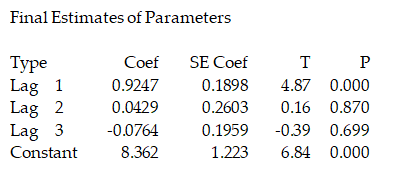
Monthly closing stock prices, adjusted for dividends, were obtained for Boeing Corporation from January 2006 through August 2008 (closing price on the first trading day of the month). The time series graph of these data is shown below. 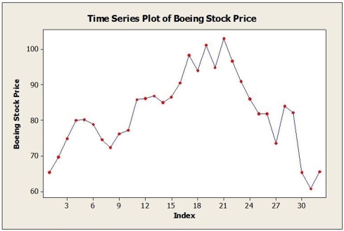 a. Below are the results of fitting a third-order autoregressive model, AR (3). Write out the model. Are the second and third lagged values significant? Explain.
Final Estimates of Parameters
Type Coef SE Coef T P
Lag 1 0.9247 0.1898 4.87 0.000
Lag 2 0.0429 0.2603 0.16 0.870
Lag 3 -0.0764 0.1959 -0.39 0.699
Constant 8.362 1.223 6.84 0.000
b. Below are the results of fitting a first-order autoregressive model, AR (1). Write out the model. Is this model typical for stock price data? Explain.
Final Estimates of Parameters
Type Coef SE Coef T P
Lag 1 0.9098 0.0969 9.39 0.000
Constant 6.835 1.207 5.67 0.000
a. Below are the results of fitting a third-order autoregressive model, AR (3). Write out the model. Are the second and third lagged values significant? Explain.Final Estimates of Parameters
Type Coef SE Coef T P
Lag 1 0.9247 0.1898 4.87 0.000
Lag 2 0.0429 0.2603 0.16 0.870
Lag 3 -0.0764 0.1959 -0.39 0.699
Constant 8.362 1.223 6.84 0.000
b. Below are the results of fitting a first-order autoregressive model, AR (1). Write out the model. Is this model typical for stock price data? Explain.
Final Estimates of Parameters
Type Coef SE Coef T P
Lag 1 0.9098 0.0969 9.39 0.000
Constant 6.835 1.207 5.67 0.000
Question
Consider the following to answer the question(s) below:
A third-order autoregressive model, AR (3) was fit to monthly closing stock prices, adjusted for dividends, of Boeing Corporation from January 2006 through August 2008 (closing price on the first trading day of the month). The results are as follows:
Let Boeing stock price be dependent variable y. The estimated model is
A) = 1.223 + 0.1898yt-1 + 0.2603yt-2 + 0.1959yt-3.
B) = 8.362 - 0.0764yt-1 + 0.0429yt-2 + 0.9247yt-3.
C) = 1.223 + 0.1959yt-1 + 0.2603yt-2 + 0.1898yt-3.
D) = 8.362 + 0.9247yt-1 + 0.0429yt-2 - 0.0764yt-3.
E) = 0.9247yt-1 + 0.2603yt-2 - 0.39yt-3.
A third-order autoregressive model, AR (3) was fit to monthly closing stock prices, adjusted for dividends, of Boeing Corporation from January 2006 through August 2008 (closing price on the first trading day of the month). The results are as follows:
Let Boeing stock price be dependent variable y. The estimated model is
A)
= 1.223 + 0.1898yt-1 + 0.2603yt-2 + 0.1959yt-3.B)
= 8.362 - 0.0764yt-1 + 0.0429yt-2 + 0.9247yt-3.C)
= 1.223 + 0.1959yt-1 + 0.2603yt-2 + 0.1898yt-3.D)
= 8.362 + 0.9247yt-1 + 0.0429yt-2 - 0.0764yt-3.E)
= 0.9247yt-1 + 0.2603yt-2 - 0.39yt-3. Question
A large automobile parts supplier keeps track of the demand for a particular part needed by its customers, automobile manufacturers. The time series plot below shows monthly demand for this part (in thousands) for a five-year period. The dominant component(s) in this time series is(are) 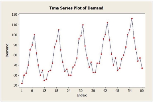
A) cyclical.
B) irregular.
C) seasonal and trend.
D) cyclical and irregular.
E) No time series component is dominant. The time series is random walk.
A) cyclical.
B) irregular.
C) seasonal and trend.
D) cyclical and irregular.
E) No time series component is dominant. The time series is random walk.
Question
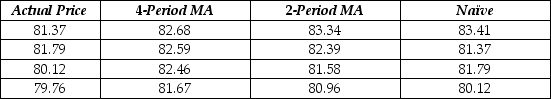
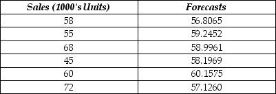
The table below shows the closing daily stock prices for Kyopera Corporation for September 2 through September 5, 2016, as well as 4-day moving average, 2-day moving average and naïve forecasts. Calculate the MAD and MSE for each of the three types of forecasts. Which is the best?
Question
Consider the following to answer the question(s) below:
A third-order autoregressive model, AR (3) was fit to monthly closing stock prices, adjusted for dividends, of Boeing Corporation from January 2006 through August 2008 (closing price on the first trading day of the month). The results are as follows:
Assume that the year 2000 is used as the index base period and that sales were $12 million in the year 2000. If sales were $18 million in the year 2006, the simple index number for the year 2006 is
A) 150.0.
B) 15.0.
C) 0.667.
D) 6 million.
E) 66.67.
Question
Consider the following to answer the question(s) below:
Annual estimates of the population in a certain city from 2005 (t = 1) onward are shown in the time series graph below.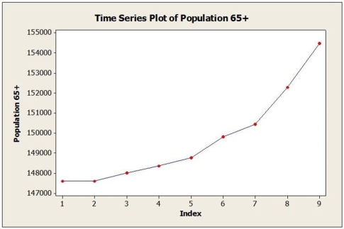
The forecasting method that will most likely be best for this time series is
A) single exponential smoothing with α = 0.1.
B) quadratic trend.
C) moving average with L = 2.
D) naïve.
E) linear trend.
Question
Daily closing stock prices for Kyopera Corporation were obtained from August 3, 2016 through August 23, 2016 and appear in the time series graph below. 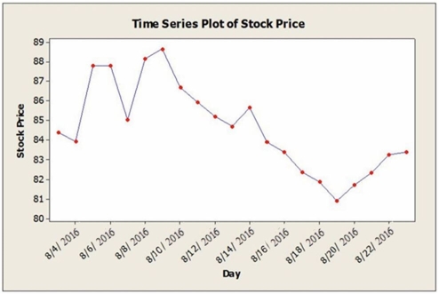 a. Identify the dominant time series component(s) in the data.
b. The method of moving averages was applied to these data. Below are time series graphs showing moving average results using two different values of L. In which application is a larger value of L used?
i.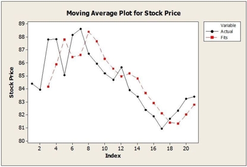 ii.
ii. 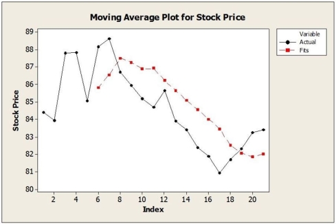 c. Suppose that the single exponential smoothing (SES) model was applied to these data. Below are time series graphs showing SES results using two different smoothing constants (α = 0.2 and α = 0.8). In which application is a larger value of α used?
i.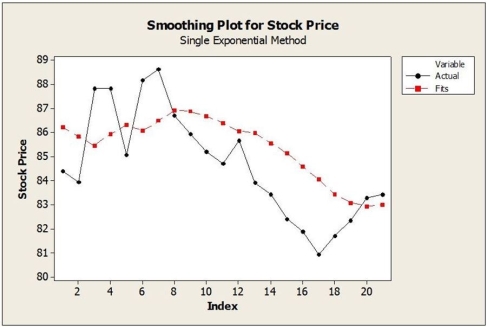 ii.
ii. 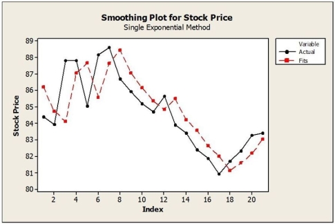
a. Identify the dominant time series component(s) in the data.b. The method of moving averages was applied to these data. Below are time series graphs showing moving average results using two different values of L. In which application is a larger value of L used?
i.
ii. c. Suppose that the single exponential smoothing (SES) model was applied to these data. Below are time series graphs showing SES results using two different smoothing constants (α = 0.2 and α = 0.8). In which application is a larger value of α used?i.
ii. Question
Consider the following to answer the question(s) below:
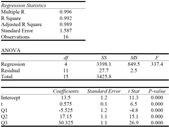
Quarterly sales data (in $10,000) for a small company specializing in green cleaning products are shown in the time series graph below. A seasonal regression model was fit to these data and the results are shown below.
The regression equation is Sales = 89.06 + 1.37t - 23.37Q2 - 23.91Q3 + 27.88Q4.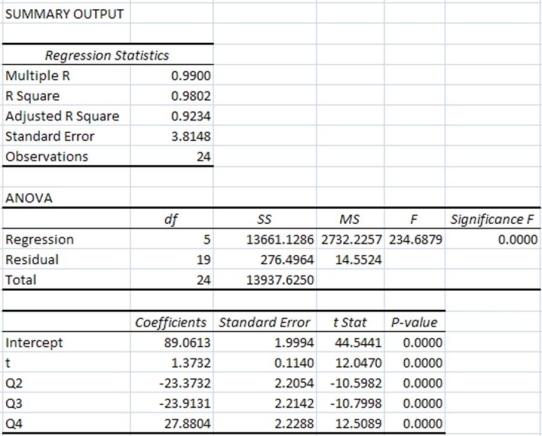
The regression coefficients in the seasonal regression model indicate that
A) sales are, on average, lower in the first, second and third quarters compared with the fourth quarter.
B) sales are, on average, lowest in the fourth quarter.
C) sales are, on average, higher in the first, second and third quarters compared with the fourth quarter.
D) sales are, on average, lowest in the first quarter.
E) sales are, on average, lowest in the third quarter.
Quarterly sales data (in $10,000) for a small company specializing in green cleaning products are shown in the time series graph below.
A seasonal regression model was fit to these data and the results are shown below.The regression equation is Sales = 89.06 + 1.37t - 23.37Q2 - 23.91Q3 + 27.88Q4.
The regression coefficients in the seasonal regression model indicate that
A) sales are, on average, lower in the first, second and third quarters compared with the fourth quarter.
B) sales are, on average, lowest in the fourth quarter.
C) sales are, on average, higher in the first, second and third quarters compared with the fourth quarter.
D) sales are, on average, lowest in the first quarter.
E) sales are, on average, lowest in the third quarter.
Question
Consider the following to answer the question(s) below:
A third-order autoregressive model, AR (3) was fit to monthly closing stock prices, adjusted for dividends, of Boeing Corporation from January 2006 through August 2008 (closing price on the first trading day of the month). The results are as follows:
Which of the following statements is true?
A) At α = 0.05, the first lagged variable is significant.
B) At α = 0.05, the second lagged variable is significant.
C) At α = 0.05, the third lagged variable is significant.
D) At α = 0.05, the second lagged variable is significant and at α = 0.05, the third lagged variable is significant.
E) At α = 0.05, the first lagged variable is not significant.
Question
Annual estimates of the population in the age group 65+ in a mid-sized city from 2005 (t = 1) onward are shown in the time series graph below. 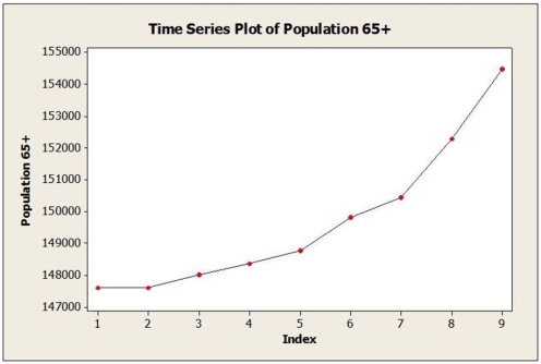 a. Identify the dominant time series component(s) in the data.
b. Below are the results from fitting a linear trend model to the data. Use this model to estimate the 65+ population in this city for 2014 (t = 10).
Fitted Trend Equation , = 145,703 + 801t
c. Below are the results from fitting a quadratic trend model to the data. Use this model to estimate the 65+ population in this city for 2014 (t = 10).
Fitted Trend Equation , = 148,187 - 554t + 135.5t2
d. The actual population estimate for 2014 is 157,218. Which model does better? Why?
a. Identify the dominant time series component(s) in the data.b. Below are the results from fitting a linear trend model to the data. Use this model to estimate the 65+ population in this city for 2014 (t = 10).
Fitted Trend Equation
, = 145,703 + 801tc. Below are the results from fitting a quadratic trend model to the data. Use this model to estimate the 65+ population in this city for 2014 (t = 10).
Fitted Trend Equation
, = 148,187 - 554t + 135.5t2d. The actual population estimate for 2014 is 157,218. Which model does better? Why?
Question
Annual estimates of the population in the age group 65+ in a certain city from 2005 (t = 1) onward are used to estimate the following quadratic trend model:  , = 148,187 - 554t + 135.5t2 Using this model, the estimate for 2014 is
A) 157,218.
B) 156,197.
C) 153,713.
D) 161,312.
E) 158,489.
, = 148,187 - 554t + 135.5t2 Using this model, the estimate for 2014 isA) 157,218.
B) 156,197.
C) 153,713.
D) 161,312.
E) 158,489.
Question
Consider the following to answer the question(s) below:
Annual estimates of the population in a certain city from 2005 (t = 1) onward are shown in the time series graph below.
The dominant component in this time series is
A) cyclical.
B) irregular.
C) seasonal.
D) trend.
E) No time series component is dominant. The time series is random walk.
Annual estimates of the population in a certain city from 2005 (t = 1) onward are shown in the time series graph below.
The dominant component in this time series is
A) cyclical.
B) irregular.
C) seasonal.
D) trend.
E) No time series component is dominant. The time series is random walk.
Question
Consider the following to answer the question(s) below:
The following table shows actual sales values and forecasts.
The MAD for the forecasting method used is
A) 7.112.
B) 9.187.
C) 82.656.
D) 113.899.
E) 8.534.
The following table shows actual sales values and forecasts.
The MAD for the forecasting method used is
A) 7.112.
B) 9.187.
C) 82.656.
D) 113.899.
E) 8.534.
Question
Quarterly sales data (in $10,000) for a small company specializing in green cleaning products are shown in the time series graph below. 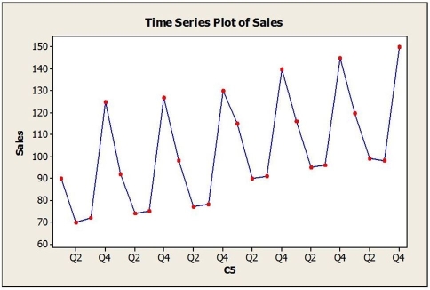 A seasonal regression model was fit to these data and the results are shown below.
The regression equation is Sales = 89.06 + 1.37t - 23.37Q2 - 23.91Q3 + 27.88Q4.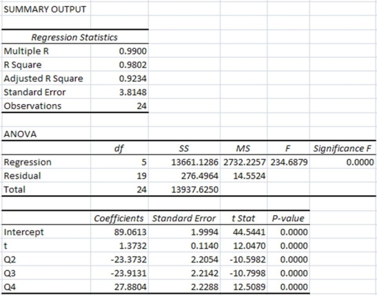 a. Is the seasonal regression model significant overall? Explain.
b. Interpret the regression coefficients in this model.
c. Use this model to provide forecasts for each of the four quarters of the next year.
A seasonal regression model was fit to these data and the results are shown below.The regression equation is Sales = 89.06 + 1.37t - 23.37Q2 - 23.91Q3 + 27.88Q4.
a. Is the seasonal regression model significant overall? Explain.b. Interpret the regression coefficients in this model.
c. Use this model to provide forecasts for each of the four quarters of the next year.
Question
Question
The following table shows actual sales values and forecasts provided by two different methods.
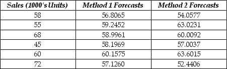 a. Calculate the MAD for each method.
b. Calculate the MSE for each method.
c. Which method forecasts better?
a. Calculate the MAD for each method.b. Calculate the MSE for each method.
c. Which method forecasts better?
Question
Annual estimates of the population in a certain city from 2004 (t = 1) onward are shown in the time series graph below. 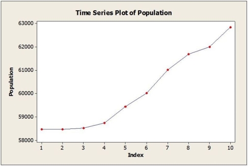 a. Identify the dominant time series component(s) in the data.
b. Below are the results from fitting a linear trend model to the data. Use this model to estimate the population in this city for 2014 (t = 11).
Fitted Trend Equation , = 57,206 + 528t
c. Below are the results from fitting a quadratic trend model to the data. Use this model to estimate the population in this city for 2014 (t = 11).
Fitted Trend Equation , = 58,159 + 52t + 43.3t2
d. The actual population estimate for 2014 is 63,828. Which model does better? Why?
a. Identify the dominant time series component(s) in the data.b. Below are the results from fitting a linear trend model to the data. Use this model to estimate the population in this city for 2014 (t = 11).
Fitted Trend Equation
, = 57,206 + 528tc. Below are the results from fitting a quadratic trend model to the data. Use this model to estimate the population in this city for 2014 (t = 11).
Fitted Trend Equation
, = 58,159 + 52t + 43.3t2d. The actual population estimate for 2014 is 63,828. Which model does better? Why?
Question
A large automobile parts supplier keeps track of the demand for a particular part needed by its customers, automobile manufacturers. The time series plot below shows monthly demand for this part (in thousands) for a five year period. 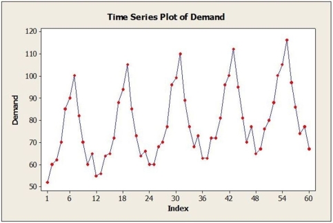 a. Identify the dominant time series component(s) in the data.
b. Suppose that the single exponential smoothing (SES) model was applied to these data. Below are time series graphs showing SES results using two different smoothing constants (α = 0.2 and α = 0.8). In which application is a larger value of α used?
i.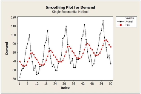 ii.
ii. 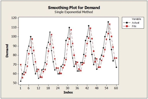 c. What forecasting method may be a better choice than SES for these data? Explain.
a. Identify the dominant time series component(s) in the data.b. Suppose that the single exponential smoothing (SES) model was applied to these data. Below are time series graphs showing SES results using two different smoothing constants (α = 0.2 and α = 0.8). In which application is a larger value of α used?
i.
ii. c. What forecasting method may be a better choice than SES for these data? Explain. Question
Consider the following to answer the question(s) below:
Quarterly sales data (in $10,000) for a small company specializing in green cleaning products are shown in the time series graph below. A seasonal regression model was fit to these data and the results are shown below.
The regression equation is Sales = 89.06 + 1.37t - 23.37Q2 - 23.91Q3 + 27.88Q4.
Which of the following is not true?
A) The seasonal regression model is significant in explaining sales as indicated by the F-statistic and associated P-value.
B) The seasonal regression model explains 98.02% of the variation in sales.
C) The t-statistics and associated P-values indicate that all dummy variables representing quarters are significant.
D) Q1 is the quarter without dummy variable. The next year sales in Q1 is predicted to be $1,233,100.
E) The seasonal regression model is not significant overall as only Q1 is significant.
Quarterly sales data (in $10,000) for a small company specializing in green cleaning products are shown in the time series graph below.
A seasonal regression model was fit to these data and the results are shown below.The regression equation is Sales = 89.06 + 1.37t - 23.37Q2 - 23.91Q3 + 27.88Q4.
Which of the following is not true?
A) The seasonal regression model is significant in explaining sales as indicated by the F-statistic and associated P-value.
B) The seasonal regression model explains 98.02% of the variation in sales.
C) The t-statistics and associated P-values indicate that all dummy variables representing quarters are significant.
D) Q1 is the quarter without dummy variable. The next year sales in Q1 is predicted to be $1,233,100.
E) The seasonal regression model is not significant overall as only Q1 is significant.
Question
Consider the following to answer the question(s) below:
A third-order autoregressive model, AR (3) was fit to monthly closing stock prices, adjusted for dividends, of Boeing Corporation from January 2006 through August 2008 (closing price on the first trading day of the month). The results are as follows:
Which of the following is true about index numbers? Index numbers are
A) used to make a relative comparison of different time periods.
B) used to measure the trend component.
C) used to measure the seasonal component.
D) used to measure the cyclical component.
E) used to measure the irregular component.
Question
A company has recorded annual sales (in $thousands) for the past 14 years and found the following linear trend model:  = 5.23 + 144.60 t. This means that
A) on average, sales are increasing by $144.6K per year.
B) on average, sales are increasing by $5.23K per year.
C) there is a seasonal component in the data.
D) sales in year one were $5.23K.
E) there is a cyclical component in the data.
= 5.23 + 144.60 t. This means thatA) on average, sales are increasing by $144.6K per year.
B) on average, sales are increasing by $5.23K per year.
C) there is a seasonal component in the data.
D) sales in year one were $5.23K.
E) there is a cyclical component in the data.
Question
Consider the following to answer the question(s) below:
A company has developed a linear trend model to forecast monthly sales. The following data show the actual sales and the "fitted" sales for months 1-12.
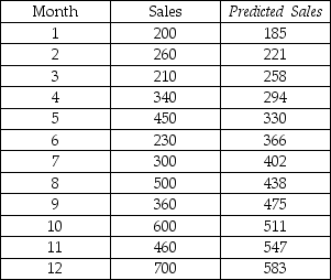
Based on these data, what is the mean absolute deviation (MAD) for the linear trend model?
A) 81.33
B) 7976.167
C) 976
D) 95714
E) 115
A company has developed a linear trend model to forecast monthly sales. The following data show the actual sales and the "fitted" sales for months 1-12.
Based on these data, what is the mean absolute deviation (MAD) for the linear trend model?
A) 81.33
B) 7976.167
C) 976
D) 95714
E) 115
Question
Question
Consider the following to answer the question(s) below:
A company has developed a linear trend model to forecast monthly sales. The following data show the actual sales and the "fitted" sales for months 1-12.
Based on these data, what is the mean absolute percentage error (MAPE) for the linear trend model?
A) 22.79
B) 81.33
C) 2.73
D) 796
E) 0.22
A company has developed a linear trend model to forecast monthly sales. The following data show the actual sales and the "fitted" sales for months 1-12.
Based on these data, what is the mean absolute percentage error (MAPE) for the linear trend model?
A) 22.79
B) 81.33
C) 2.73
D) 796
E) 0.22
Question
Question
A time series is shown below. Perform single exponential smoothing for this data set using α = 0.2. What is the value of the forecast for period 6? 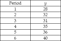
A) 31.5
B) 33.2
C) 36
D) 40
E) 30.4
A) 31.5
B) 33.2
C) 36
D) 40
E) 30.4
Question
Consider the following to answer the question(s) below:
The quarterly sales of all types of bicycles sold at a small sporting goods store in Charlottetown for the 16 quarters from January 2012 to December 2015 are depicted in the time series graph below.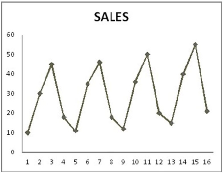
Which of the following statements do not describe this data and model?
A) The seasonal component is the most dominant.
B) All of the coefficients are significant for α = 0.05.
C) The model is additive.
D) The regression model has both trend and seasonal components.
E) The regression model has no dummy variables.
Question
Consider the following to answer the question(s) below:
A company has developed a linear trend model to forecast monthly sales. The following data show the actual sales and the "fitted" sales for months 1-12.
Based on these data, what is the mean square error (MSE) for the linear trend model?
A) 7976.167
B) 95714
C) 81.33
D) 976
E) 8701.273
A company has developed a linear trend model to forecast monthly sales. The following data show the actual sales and the "fitted" sales for months 1-12.
Based on these data, what is the mean square error (MSE) for the linear trend model?
A) 7976.167
B) 95714
C) 81.33
D) 976
E) 8701.273

Unlock Deck
Sign up to unlock the cards in this deck!
Unlock Deck
Unlock Deck
1/28
Play
Full screen (f)
Deck 22: Time Series Analysis
1
Monthly closing stock prices, adjusted for dividends, were obtained for Boeing Corporation from January 2006 through August 2008 (closing price on the first trading day of the month). The time series graph of these data is shown below. a. Below are the results of fitting a third-order autoregressive model, AR (3). Write out the model. Are the second and third lagged values significant? Explain.
Final Estimates of Parameters
Type Coef SE Coef T P
Lag 1 0.9247 0.1898 4.87 0.000
Lag 2 0.0429 0.2603 0.16 0.870
Lag 3 -0.0764 0.1959 -0.39 0.699
Constant 8.362 1.223 6.84 0.000
b. Below are the results of fitting a first-order autoregressive model, AR (1). Write out the model. Is this model typical for stock price data? Explain.
Final Estimates of Parameters
Type Coef SE Coef T P
Lag 1 0.9098 0.0969 9.39 0.000
Constant 6.835 1.207 5.67 0.000
a. Below are the results of fitting a third-order autoregressive model, AR (3). Write out the model. Are the second and third lagged values significant? Explain.Final Estimates of Parameters
Type Coef SE Coef T P
Lag 1 0.9247 0.1898 4.87 0.000
Lag 2 0.0429 0.2603 0.16 0.870
Lag 3 -0.0764 0.1959 -0.39 0.699
Constant 8.362 1.223 6.84 0.000
b. Below are the results of fitting a first-order autoregressive model, AR (1). Write out the model. Is this model typical for stock price data? Explain.
Final Estimates of Parameters
Type Coef SE Coef T P
Lag 1 0.9098 0.0969 9.39 0.000
Constant 6.835 1.207 5.67 0.000
Let Boeing stock price be dependent variable y.
a. = 8.362 + 0.9247yt-1 + 0.0429yt-2 - 0.0764yt-3
The second and third lagged values are not significant, as can be seen by their relatively large
P-values (0.870 and 0.699, respectively).
b. = 6.835 + 0.9098yt-1
With a relatively large Lag 1 coefficient, this is similar to what we find with stock price data. However, the values are monthly and not daily, so they are not as volatile and less likely to be a random walk. In addition, the estimated intercept is not close to zero.
a.
= 8.362 + 0.9247yt-1 + 0.0429yt-2 - 0.0764yt-3The second and third lagged values are not significant, as can be seen by their relatively large
P-values (0.870 and 0.699, respectively).
b.
= 6.835 + 0.9098yt-1With a relatively large Lag 1 coefficient, this is similar to what we find with stock price data. However, the values are monthly and not daily, so they are not as volatile and less likely to be a random walk. In addition, the estimated intercept is not close to zero.
2
Consider the following to answer the question(s) below:
A third-order autoregressive model, AR (3) was fit to monthly closing stock prices, adjusted for dividends, of Boeing Corporation from January 2006 through August 2008 (closing price on the first trading day of the month). The results are as follows:
Let Boeing stock price be dependent variable y. The estimated model is
A) = 1.223 + 0.1898yt-1 + 0.2603yt-2 + 0.1959yt-3.
B) = 8.362 - 0.0764yt-1 + 0.0429yt-2 + 0.9247yt-3.
C) = 1.223 + 0.1959yt-1 + 0.2603yt-2 + 0.1898yt-3.
D) = 8.362 + 0.9247yt-1 + 0.0429yt-2 - 0.0764yt-3.
E) = 0.9247yt-1 + 0.2603yt-2 - 0.39yt-3.
A third-order autoregressive model, AR (3) was fit to monthly closing stock prices, adjusted for dividends, of Boeing Corporation from January 2006 through August 2008 (closing price on the first trading day of the month). The results are as follows:
Let Boeing stock price be dependent variable y. The estimated model is
A)
= 1.223 + 0.1898yt-1 + 0.2603yt-2 + 0.1959yt-3.B)
= 8.362 - 0.0764yt-1 + 0.0429yt-2 + 0.9247yt-3.C)
= 1.223 + 0.1959yt-1 + 0.2603yt-2 + 0.1898yt-3.D)
= 8.362 + 0.9247yt-1 + 0.0429yt-2 - 0.0764yt-3.E)
= 0.9247yt-1 + 0.2603yt-2 - 0.39yt-3. = 8.362 + 0.9247yt-1 + 0.0429yt-2 - 0.0764yt-3. 3
A large automobile parts supplier keeps track of the demand for a particular part needed by its customers, automobile manufacturers. The time series plot below shows monthly demand for this part (in thousands) for a five-year period. The dominant component(s) in this time series is(are)
A) cyclical.
B) irregular.
C) seasonal and trend.
D) cyclical and irregular.
E) No time series component is dominant. The time series is random walk.
A) cyclical.
B) irregular.
C) seasonal and trend.
D) cyclical and irregular.
E) No time series component is dominant. The time series is random walk.
seasonal and trend.
4
The table below shows the closing daily stock prices for Kyopera Corporation for September 2 through September 5, 2016, as well as 4-day moving average, 2-day moving average and naïve forecasts. Calculate the MAD and MSE for each of the three types of forecasts. Which is the best?
Unlock Deck
Unlock for access to all 28 flashcards in this deck.
Unlock Deck
k this deck
5
Consider the following to answer the question(s) below:
A third-order autoregressive model, AR (3) was fit to monthly closing stock prices, adjusted for dividends, of Boeing Corporation from January 2006 through August 2008 (closing price on the first trading day of the month). The results are as follows:
Assume that the year 2000 is used as the index base period and that sales were $12 million in the year 2000. If sales were $18 million in the year 2006, the simple index number for the year 2006 is
A) 150.0.
B) 15.0.
C) 0.667.
D) 6 million.
E) 66.67.
Unlock Deck
Unlock for access to all 28 flashcards in this deck.
Unlock Deck
k this deck
6
Consider the following to answer the question(s) below:
Annual estimates of the population in a certain city from 2005 (t = 1) onward are shown in the time series graph below.
The forecasting method that will most likely be best for this time series is
A) single exponential smoothing with α = 0.1.
B) quadratic trend.
C) moving average with L = 2.
D) naïve.
E) linear trend.
Unlock Deck
Unlock for access to all 28 flashcards in this deck.
Unlock Deck
k this deck
7
Daily closing stock prices for Kyopera Corporation were obtained from August 3, 2016 through August 23, 2016 and appear in the time series graph below. a. Identify the dominant time series component(s) in the data.
b. The method of moving averages was applied to these data. Below are time series graphs showing moving average results using two different values of L. In which application is a larger value of L used?
i. ii. c. Suppose that the single exponential smoothing (SES) model was applied to these data. Below are time series graphs showing SES results using two different smoothing constants (α = 0.2 and α = 0.8). In which application is a larger value of α used?
i. ii.
a. Identify the dominant time series component(s) in the data.b. The method of moving averages was applied to these data. Below are time series graphs showing moving average results using two different values of L. In which application is a larger value of L used?
i.
ii. c. Suppose that the single exponential smoothing (SES) model was applied to these data. Below are time series graphs showing SES results using two different smoothing constants (α = 0.2 and α = 0.8). In which application is a larger value of α used?i.
ii. Unlock Deck
Unlock for access to all 28 flashcards in this deck.
Unlock Deck
k this deck
8
Consider the following to answer the question(s) below:
Quarterly sales data (in $10,000) for a small company specializing in green cleaning products are shown in the time series graph below. A seasonal regression model was fit to these data and the results are shown below.
The regression equation is Sales = 89.06 + 1.37t - 23.37Q2 - 23.91Q3 + 27.88Q4.
The regression coefficients in the seasonal regression model indicate that
A) sales are, on average, lower in the first, second and third quarters compared with the fourth quarter.
B) sales are, on average, lowest in the fourth quarter.
C) sales are, on average, higher in the first, second and third quarters compared with the fourth quarter.
D) sales are, on average, lowest in the first quarter.
E) sales are, on average, lowest in the third quarter.
Quarterly sales data (in $10,000) for a small company specializing in green cleaning products are shown in the time series graph below.
A seasonal regression model was fit to these data and the results are shown below.The regression equation is Sales = 89.06 + 1.37t - 23.37Q2 - 23.91Q3 + 27.88Q4.
The regression coefficients in the seasonal regression model indicate that
A) sales are, on average, lower in the first, second and third quarters compared with the fourth quarter.
B) sales are, on average, lowest in the fourth quarter.
C) sales are, on average, higher in the first, second and third quarters compared with the fourth quarter.
D) sales are, on average, lowest in the first quarter.
E) sales are, on average, lowest in the third quarter.
Unlock Deck
Unlock for access to all 28 flashcards in this deck.
Unlock Deck
k this deck
9
Consider the following to answer the question(s) below:
A third-order autoregressive model, AR (3) was fit to monthly closing stock prices, adjusted for dividends, of Boeing Corporation from January 2006 through August 2008 (closing price on the first trading day of the month). The results are as follows:
Which of the following statements is true?
A) At α = 0.05, the first lagged variable is significant.
B) At α = 0.05, the second lagged variable is significant.
C) At α = 0.05, the third lagged variable is significant.
D) At α = 0.05, the second lagged variable is significant and at α = 0.05, the third lagged variable is significant.
E) At α = 0.05, the first lagged variable is not significant.
Unlock Deck
Unlock for access to all 28 flashcards in this deck.
Unlock Deck
k this deck
10
Annual estimates of the population in the age group 65+ in a mid-sized city from 2005 (t = 1) onward are shown in the time series graph below. a. Identify the dominant time series component(s) in the data.
b. Below are the results from fitting a linear trend model to the data. Use this model to estimate the 65+ population in this city for 2014 (t = 10).
Fitted Trend Equation , = 145,703 + 801t
c. Below are the results from fitting a quadratic trend model to the data. Use this model to estimate the 65+ population in this city for 2014 (t = 10).
Fitted Trend Equation , = 148,187 - 554t + 135.5t2
d. The actual population estimate for 2014 is 157,218. Which model does better? Why?
a. Identify the dominant time series component(s) in the data.b. Below are the results from fitting a linear trend model to the data. Use this model to estimate the 65+ population in this city for 2014 (t = 10).
Fitted Trend Equation
, = 145,703 + 801tc. Below are the results from fitting a quadratic trend model to the data. Use this model to estimate the 65+ population in this city for 2014 (t = 10).
Fitted Trend Equation
, = 148,187 - 554t + 135.5t2d. The actual population estimate for 2014 is 157,218. Which model does better? Why?
Unlock Deck
Unlock for access to all 28 flashcards in this deck.
Unlock Deck
k this deck
11
Annual estimates of the population in the age group 65+ in a certain city from 2005 (t = 1) onward are used to estimate the following quadratic trend model: , = 148,187 - 554t + 135.5t2 Using this model, the estimate for 2014 is
A) 157,218.
B) 156,197.
C) 153,713.
D) 161,312.
E) 158,489.
, = 148,187 - 554t + 135.5t2 Using this model, the estimate for 2014 isA) 157,218.
B) 156,197.
C) 153,713.
D) 161,312.
E) 158,489.
Unlock Deck
Unlock for access to all 28 flashcards in this deck.
Unlock Deck
k this deck
12
Consider the following to answer the question(s) below:
Annual estimates of the population in a certain city from 2005 (t = 1) onward are shown in the time series graph below.
The dominant component in this time series is
A) cyclical.
B) irregular.
C) seasonal.
D) trend.
E) No time series component is dominant. The time series is random walk.
Annual estimates of the population in a certain city from 2005 (t = 1) onward are shown in the time series graph below.
The dominant component in this time series is
A) cyclical.
B) irregular.
C) seasonal.
D) trend.
E) No time series component is dominant. The time series is random walk.
Unlock Deck
Unlock for access to all 28 flashcards in this deck.
Unlock Deck
k this deck
13
Consider the following to answer the question(s) below:
The following table shows actual sales values and forecasts.
The MAD for the forecasting method used is
A) 7.112.
B) 9.187.
C) 82.656.
D) 113.899.
E) 8.534.
The following table shows actual sales values and forecasts.
The MAD for the forecasting method used is
A) 7.112.
B) 9.187.
C) 82.656.
D) 113.899.
E) 8.534.
Unlock Deck
Unlock for access to all 28 flashcards in this deck.
Unlock Deck
k this deck
14
Quarterly sales data (in $10,000) for a small company specializing in green cleaning products are shown in the time series graph below. A seasonal regression model was fit to these data and the results are shown below.
The regression equation is Sales = 89.06 + 1.37t - 23.37Q2 - 23.91Q3 + 27.88Q4. a. Is the seasonal regression model significant overall? Explain.
b. Interpret the regression coefficients in this model.
c. Use this model to provide forecasts for each of the four quarters of the next year.
A seasonal regression model was fit to these data and the results are shown below.The regression equation is Sales = 89.06 + 1.37t - 23.37Q2 - 23.91Q3 + 27.88Q4.
a. Is the seasonal regression model significant overall? Explain.b. Interpret the regression coefficients in this model.
c. Use this model to provide forecasts for each of the four quarters of the next year.
Unlock Deck
Unlock for access to all 28 flashcards in this deck.
Unlock Deck
k this deck
15
The MSE for the forecasting method used is
A) 7.112.
B) 9.187.
C) 82.656.
D) 113.899.
E) 99.187.
A) 7.112.
B) 9.187.
C) 82.656.
D) 113.899.
E) 99.187.
Unlock Deck
Unlock for access to all 28 flashcards in this deck.
Unlock Deck
k this deck
16
The following table shows actual sales values and forecasts provided by two different methods.
a. Calculate the MAD for each method.
b. Calculate the MSE for each method.
c. Which method forecasts better?
a. Calculate the MAD for each method.b. Calculate the MSE for each method.
c. Which method forecasts better?
Unlock Deck
Unlock for access to all 28 flashcards in this deck.
Unlock Deck
k this deck
17
Annual estimates of the population in a certain city from 2004 (t = 1) onward are shown in the time series graph below. a. Identify the dominant time series component(s) in the data.
b. Below are the results from fitting a linear trend model to the data. Use this model to estimate the population in this city for 2014 (t = 11).
Fitted Trend Equation , = 57,206 + 528t
c. Below are the results from fitting a quadratic trend model to the data. Use this model to estimate the population in this city for 2014 (t = 11).
Fitted Trend Equation , = 58,159 + 52t + 43.3t2
d. The actual population estimate for 2014 is 63,828. Which model does better? Why?
a. Identify the dominant time series component(s) in the data.b. Below are the results from fitting a linear trend model to the data. Use this model to estimate the population in this city for 2014 (t = 11).
Fitted Trend Equation
, = 57,206 + 528tc. Below are the results from fitting a quadratic trend model to the data. Use this model to estimate the population in this city for 2014 (t = 11).
Fitted Trend Equation
, = 58,159 + 52t + 43.3t2d. The actual population estimate for 2014 is 63,828. Which model does better? Why?
Unlock Deck
Unlock for access to all 28 flashcards in this deck.
Unlock Deck
k this deck
18
A large automobile parts supplier keeps track of the demand for a particular part needed by its customers, automobile manufacturers. The time series plot below shows monthly demand for this part (in thousands) for a five year period. a. Identify the dominant time series component(s) in the data.
b. Suppose that the single exponential smoothing (SES) model was applied to these data. Below are time series graphs showing SES results using two different smoothing constants (α = 0.2 and α = 0.8). In which application is a larger value of α used?
i. ii. c. What forecasting method may be a better choice than SES for these data? Explain.
a. Identify the dominant time series component(s) in the data.b. Suppose that the single exponential smoothing (SES) model was applied to these data. Below are time series graphs showing SES results using two different smoothing constants (α = 0.2 and α = 0.8). In which application is a larger value of α used?
i.
ii. c. What forecasting method may be a better choice than SES for these data? Explain. Unlock Deck
Unlock for access to all 28 flashcards in this deck.
Unlock Deck
k this deck
19
Consider the following to answer the question(s) below:
Quarterly sales data (in $10,000) for a small company specializing in green cleaning products are shown in the time series graph below. A seasonal regression model was fit to these data and the results are shown below.
The regression equation is Sales = 89.06 + 1.37t - 23.37Q2 - 23.91Q3 + 27.88Q4.
Which of the following is not true?
A) The seasonal regression model is significant in explaining sales as indicated by the F-statistic and associated P-value.
B) The seasonal regression model explains 98.02% of the variation in sales.
C) The t-statistics and associated P-values indicate that all dummy variables representing quarters are significant.
D) Q1 is the quarter without dummy variable. The next year sales in Q1 is predicted to be $1,233,100.
E) The seasonal regression model is not significant overall as only Q1 is significant.
Quarterly sales data (in $10,000) for a small company specializing in green cleaning products are shown in the time series graph below.
A seasonal regression model was fit to these data and the results are shown below.The regression equation is Sales = 89.06 + 1.37t - 23.37Q2 - 23.91Q3 + 27.88Q4.
Which of the following is not true?
A) The seasonal regression model is significant in explaining sales as indicated by the F-statistic and associated P-value.
B) The seasonal regression model explains 98.02% of the variation in sales.
C) The t-statistics and associated P-values indicate that all dummy variables representing quarters are significant.
D) Q1 is the quarter without dummy variable. The next year sales in Q1 is predicted to be $1,233,100.
E) The seasonal regression model is not significant overall as only Q1 is significant.
Unlock Deck
Unlock for access to all 28 flashcards in this deck.
Unlock Deck
k this deck
20
Consider the following to answer the question(s) below:
A third-order autoregressive model, AR (3) was fit to monthly closing stock prices, adjusted for dividends, of Boeing Corporation from January 2006 through August 2008 (closing price on the first trading day of the month). The results are as follows:
Which of the following is true about index numbers? Index numbers are
A) used to make a relative comparison of different time periods.
B) used to measure the trend component.
C) used to measure the seasonal component.
D) used to measure the cyclical component.
E) used to measure the irregular component.
Unlock Deck
Unlock for access to all 28 flashcards in this deck.
Unlock Deck
k this deck
21
A company has recorded annual sales (in $thousands) for the past 14 years and found the following linear trend model: = 5.23 + 144.60 t. This means that
A) on average, sales are increasing by $144.6K per year.
B) on average, sales are increasing by $5.23K per year.
C) there is a seasonal component in the data.
D) sales in year one were $5.23K.
E) there is a cyclical component in the data.
= 5.23 + 144.60 t. This means thatA) on average, sales are increasing by $144.6K per year.
B) on average, sales are increasing by $5.23K per year.
C) there is a seasonal component in the data.
D) sales in year one were $5.23K.
E) there is a cyclical component in the data.
Unlock Deck
Unlock for access to all 28 flashcards in this deck.
Unlock Deck
k this deck
22
Consider the following to answer the question(s) below:
A company has developed a linear trend model to forecast monthly sales. The following data show the actual sales and the "fitted" sales for months 1-12.
Based on these data, what is the mean absolute deviation (MAD) for the linear trend model?
A) 81.33
B) 7976.167
C) 976
D) 95714
E) 115
A company has developed a linear trend model to forecast monthly sales. The following data show the actual sales and the "fitted" sales for months 1-12.
Based on these data, what is the mean absolute deviation (MAD) for the linear trend model?
A) 81.33
B) 7976.167
C) 976
D) 95714
E) 115
Unlock Deck
Unlock for access to all 28 flashcards in this deck.
Unlock Deck
k this deck
23
Which of the following statement is true about statistical measures used to estimate and report forecast error?
A) MSE (mean square error) is in the same units as the data.
B) MAD (mean absolute deviation) can be negative.
C) If the measurements are rescaled, MAD won't change.
D) Forecast errors cannot be negative.
E) If you choose to rescale measurements, both MASE and MAD will change, but MAPE will remain the same.
Unlock Deck
Unlock for access to all 28 flashcards in this deck.
Unlock Deck
k this deck
24
Consider the following to answer the question(s) below:
A company has developed a linear trend model to forecast monthly sales. The following data show the actual sales and the "fitted" sales for months 1-12.
Based on these data, what is the mean absolute percentage error (MAPE) for the linear trend model?
A) 22.79
B) 81.33
C) 2.73
D) 796
E) 0.22
A company has developed a linear trend model to forecast monthly sales. The following data show the actual sales and the "fitted" sales for months 1-12.
Based on these data, what is the mean absolute percentage error (MAPE) for the linear trend model?
A) 22.79
B) 81.33
C) 2.73
D) 796
E) 0.22
Unlock Deck
Unlock for access to all 28 flashcards in this deck.
Unlock Deck
k this deck
25
If you suspect that your trend forecasting model may have autocorrelated forecast errors, it is appropriate to compute
A) the Durbin-Watson test statistic.
B) the MAD.
C) the MSE.
D) the MAPE.
E) the correlation coefficient.
A) the Durbin-Watson test statistic.
B) the MAD.
C) the MSE.
D) the MAPE.
E) the correlation coefficient.
Unlock Deck
Unlock for access to all 28 flashcards in this deck.
Unlock Deck
k this deck
26
A time series is shown below. Perform single exponential smoothing for this data set using α = 0.2. What is the value of the forecast for period 6?
A) 31.5
B) 33.2
C) 36
D) 40
E) 30.4
A) 31.5
B) 33.2
C) 36
D) 40
E) 30.4
Unlock Deck
Unlock for access to all 28 flashcards in this deck.
Unlock Deck
k this deck
27
Consider the following to answer the question(s) below:
The quarterly sales of all types of bicycles sold at a small sporting goods store in Charlottetown for the 16 quarters from January 2012 to December 2015 are depicted in the time series graph below.
Which of the following statements do not describe this data and model?
A) The seasonal component is the most dominant.
B) All of the coefficients are significant for α = 0.05.
C) The model is additive.
D) The regression model has both trend and seasonal components.
E) The regression model has no dummy variables.
Unlock Deck
Unlock for access to all 28 flashcards in this deck.
Unlock Deck
k this deck
28
Consider the following to answer the question(s) below:
A company has developed a linear trend model to forecast monthly sales. The following data show the actual sales and the "fitted" sales for months 1-12.
Based on these data, what is the mean square error (MSE) for the linear trend model?
A) 7976.167
B) 95714
C) 81.33
D) 976
E) 8701.273
A company has developed a linear trend model to forecast monthly sales. The following data show the actual sales and the "fitted" sales for months 1-12.
Based on these data, what is the mean square error (MSE) for the linear trend model?
A) 7976.167
B) 95714
C) 81.33
D) 976
E) 8701.273
Unlock Deck
Unlock for access to all 28 flashcards in this deck.
Unlock Deck
k this deck
Unlock Deck
Unlock for access to all 28 flashcards in this deck.


