Introduction to Management Science 12th Edition by Bernard Taylor

Exercise 39

For the ComputerWorld example in this chapter, recreate the simulation shown in Exhibit using Crystal Ball. Assume that demand is normally distributed with a mean of 1.5 laptops and a standard deviation of 0.8. Using Crystal Ball determine average weekly demand and average weekly revenue.
Exhibit

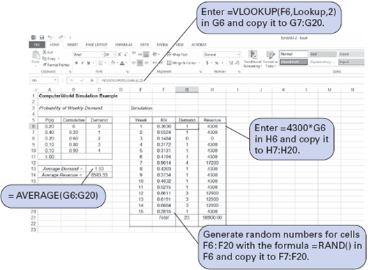
formula = A6 + B6 in cell B7, and copying this formula to cells B8:B10. This cumulative probability creates a range of random numbers for each demand value. For example, any random number less than 0.20 will result in a demand value of 0, and any random number greater than 0.20 but less than 0.60 will result in a demand value of 1, and so on. (Notice that there is no value of 1.00 in cell B11; the last demand value, 4, will be selected for any random number equal to or greater than.90.)
Random numbers are generated in cells F6:F20 by entering the formula = RAND () in cell F6 and copying it to the range of cells in F7:F20.
Now we need to be able to generate demand values for each of these random numbers in column F. We accomplish this by first covering the cumulative probabilities and the demand values in cells B6:C10 with the cursor. Then we give this range of cells the name "Lookup." This can be done by typing "Lookup" directly on the formula bar in place of B6 or by clicking on the "Insert" button at the top of the spreadsheet and selecting "Name" and "Define" and then entering the name "Lookup." This has the effect of creating a table called "Lookup" with the ranges of random numbers and associated demand values in it. Next, we enter the formula = VLOOKUP ( F6 , Lookup,2 ) in cell G6 and copy it to the cells in the range G7:G20. This formula will compare the random numbers in column F with the cumulative probabilities in B6:B10 and generate the correct demand value from cells C6:C10.
Once the demand values have been generated in column G, we can determine the weekly revenue values by entering the formula = 4300 * G6 in H6 and copying it to cells H7:H20.
Average weekly demand is computed in cell C13 by using the formula = AVERAGE (G6:G20) , and the average weekly revenue is computed by entering a similar formula in cell C14.
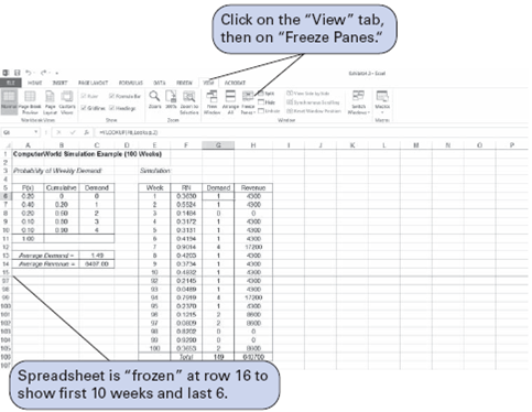
Notice that the average weekly demand value of 1.53 in Exhibit is different from the simulation result (2.07) we obtained from Table 14.4. This is because we used a different stream of random numbers. As mentioned previously, to acquire an average closer to the true steadystate value, the simulation probably needs to include more repetitions than 15 weeks. As an example, Exhibit 1 simulates demand for 100 weeks. The window has been "frozen" at row 16 and scrolled up to show the first 10 weeks and the last 6 weeks on the screen in Exhibit 1.
Exhibit 1