
An Introduction to Management Science 13th Edition by David Anderson,Dennis Sweeney ,Thomas Williams ,Jeffrey Camm, Kipp Martin
Edition 13ISBN: 978-1439043271An Introduction to Management Science 13th Edition by David Anderson,Dennis Sweeney ,Thomas Williams ,Jeffrey Camm, Kipp Martin
Edition 13ISBN: 978-1439043271 Exercise 26
Consider the following linear program: 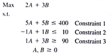
Figure 2.22 shows a graph of the constraint lines.
a. Place a number (1, 2, or 3) next to each constraint line to identify which constraint it represents.
b. Shade in the feasible region on the graph.
c. Identify the optimal extreme point. What is the optimal solution?
d. Which constraints are binding? Explain.
e. How much slack or surplus is associated with the nonbinding constraint?
Explanation Verified
Linear programming:
Linear programming ...
An Introduction to Management Science 13th Edition by David Anderson,Dennis Sweeney ,Thomas Williams ,Jeffrey Camm, Kipp Martin
Why don’t you like this exercise?
Other Minimum 8 character and maximum 255 character
Character 255


