
An Introduction to Management Science 13th Edition by David Anderson,Dennis Sweeney ,Thomas Williams ,Jeffrey Camm, Kipp Martin
Edition 13ISBN: 978-1439043271An Introduction to Management Science 13th Edition by David Anderson,Dennis Sweeney ,Thomas Williams ,Jeffrey Camm, Kipp Martin
Edition 13ISBN: 978-1439043271 Exercise 3
Consider the following linear program: 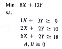
a. Use the graphical solution procedure to find the optimal solution.
b. Assume that the objective function coefficient for X changes from 8 to 6 Does the optimal solution change? Use the graphical solution procedure to find the new optimal solution.
c. Assume that the objective function coefficient for X remains 8, but the objective function coefficient for Y changes from 12 to 6. Does the optimal solution change? Use the graphical solution procedure to find the new optimal solution.
d. The computer solution for the linear program in part (a) provides the following objective coefficient range information: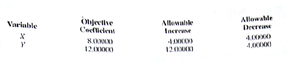
How would this objective coefficient range information help you answer parts(b) and (c) prior to re-solving the problem?
Explanation Verified
Linear Programming:
Linear programming ...
An Introduction to Management Science 13th Edition by David Anderson,Dennis Sweeney ,Thomas Williams ,Jeffrey Camm, Kipp Martin
Why don’t you like this exercise?
Other Minimum 8 character and maximum 255 character
Character 255


