
An Introduction to Management Science 13th Edition by David Anderson,Dennis Sweeney ,Thomas Williams ,Jeffrey Camm, Kipp Martin
Edition 13ISBN: 978-1439043271An Introduction to Management Science 13th Edition by David Anderson,Dennis Sweeney ,Thomas Williams ,Jeffrey Camm, Kipp Martin
Edition 13ISBN: 978-1439043271 Exercise 21
Many forecasting models use parameters that are estimated using nonlinear optimization. A good example is the Bass model introduced in this chapter. Another example is the exponential smoothing forecasting model. The exponential smoothing model is common in practice and is described in further detail in Chapter 15. For instance, the basic exponential smoothing model for forecasting sales is 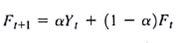
where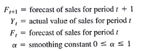
This model is used recursively; the forecast for time period t + 1 is based on the forecast for period t , F t , the observed value of sales in period t , Y t , and the smoothing parameter ?. The use of this model to forecast sales for 12 months is illustrated in Table 8.9 with the smoothing constant ? = 0.3. The forecast errors, Y t ? F t are calculated in the fourth column The value of ? is often chosen by minimizing the sum of squared forecast errors, commonly referred to as the mean squared error (MSE). The last column of Table 8.9 shows the square of the forecast error and the sum of squared forecast errors.
In using exponential smoothing models one tries to choose the value of ? that provides the best forecasts. Build an Excel Solver or LINGO optimization model that will find the smoothing parameter, ? , that minimizes the sum of forecast errors squared. You may find it easiest to put Table 8.9 into an Excel spreadsheet and then use Solver to find the optimal value of ?.
TABLE 8.9 EXPONENTIAL SMOOTHING MODEL FOR ? = 0.3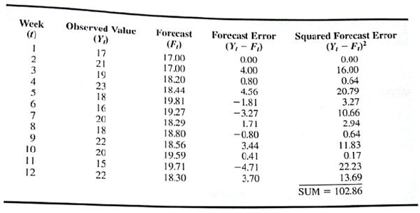
Explanation

This question doesn’t have an expert verified answer yet, let Examlex AI Copilot help.
An Introduction to Management Science 13th Edition by David Anderson,Dennis Sweeney ,Thomas Williams ,Jeffrey Camm, Kipp Martin
Why don’t you like this exercise?
Other Minimum 8 character and maximum 255 character
Character 255


