Exam 28: Consumption and the Aggregate Expenditures Model
Exam 1: Economics: the Study of Choice138 Questions
Exam 2: Confronting Scarcity: Choices in Production193 Questions
Exam 3: Demand and Supply243 Questions
Exam 4: Applications of Demand and Supply108 Questions
Exam 5: Macroeconomics: the Big Picture243 Questions
Exam 6: Measuring Total Output and Income228 Questions
Exam 7: Aggregate Demand and Aggregate Supply223 Questions
Exam 8: Economic Growth221 Questions
Exam 9: The Nature and Creation of Money267 Questions
Exam 10: Monopoly229 Questions
Exam 11: The World of Imperfect Competition227 Questions
Exam 12: Wages and Employment in Perfect Competition173 Questions
Exam 13: Interest Rates and the Markets for Capital and Natural Resources161 Questions
Exam 14: Imperfectly Competitive Markets for Factors of Production178 Questions
Exam 15: Public Finance and Public Choice179 Questions
Exam 16: Inflation and Unemployment132 Questions
Exam 17: International Trade179 Questions
Exam 18: The Economics of the Environment144 Questions
Exam 19: Inequality, Poverty, and Discrimination134 Questions
Exam 20: Macroeconomics: the Big Picture104 Questions
Exam 21: Measuring Total Income and Output134 Questions
Exam 22: Aggregate Demand and Aggregate Supply120 Questions
Exam 23: Economic Growth124 Questions
Exam 24: The Nature and Creation of Money183 Questions
Exam 25: Financial Markets and the Economy158 Questions
Exam 26: Monetary Policy and the Fed175 Questions
Exam 27: Government and Fiscal Policy177 Questions
Exam 28: Consumption and the Aggregate Expenditures Model199 Questions
Exam 29: Investment and Economic Activity115 Questions
Exam 30: Net Exports and International Finance202 Questions
Exam 31: Macro Inflation and Unemployment135 Questions
Exam 32: Macro a Brief History of Macroeconomic Thought and Policy120 Questions
Exam 33: Economic Development107 Questions
Exam 34: Socialist Economies in Transition129 Questions
Select questions type
Figure 13-3
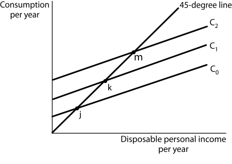 -Refer to Figure 13-3.Upward shifts of the consumption function, for example from C0 to C1 to C2 demonstrate
(Multiple Choice)
4.9/5  (36)
(36)
Let AE = Aggregate Expenditures, C = Consumption, IP = Planned Investment,
G = Government Purchases.Consider a simple aggregate expenditures model, where
AE = C + IP + G and all components of aggregate expenditures except consumption are autonomous.All other things unchanged, an increase in the price level,
(Multiple Choice)
4.8/5 (34)
In a graph with real GDP on the horizontal axis and aggregate expenditures on the vertical axis, autonomous aggregate expenditures are represented by
(Multiple Choice)
4.9/5 (36)
Figure 13-4
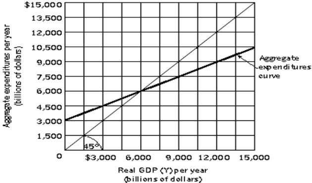 -Refer to Figure 13-4.Let Y = real GDP, AE = Aggregate Expenditures, C = Consumption,
IP = Planned Investment.Suppose AE = C + IP.IP is autonomous and the consumption function is C = $1,000 billion + 0.5Y.If real GDP = $7,000 billion, what is the amount of aggregate expenditures?
-Refer to Figure 13-4.Let Y = real GDP, AE = Aggregate Expenditures, C = Consumption,
IP = Planned Investment.Suppose AE = C + IP.IP is autonomous and the consumption function is C = $1,000 billion + 0.5Y.If real GDP = $7,000 billion, what is the amount of aggregate expenditures?
(Multiple Choice)
4.9/5 (40)
In general, an increase in the income tax rate will make the aggregate expenditures curve
(Multiple Choice)
4.7/5 (34)
Suppose the consumption function is C = $500 + 0.8Y.If Y = $1,000, then autonomous consumption is
(Multiple Choice)
4.8/5 (27)
Let AE = Aggregate Expenditures, C = Consumption, IP = Planned Investment,
G = Government Purchases.Consider a simple aggregate expenditures model, where
AE = C + IP + G and all components of aggregate expenditures except consumption are autonomous.All other things unchanged, a decrease in the price level
(Multiple Choice)
4.9/5 (33)
In the simple aggregate expenditure model where all components of aggregate expenditure are autonomous except consumption, the size of the multiplier depends on the
(Multiple Choice)
4.9/5 (36)
Aggregate expenditures that vary with real GDP are called induced aggregate expenditures.
(True/False)
4.9/5 (36)
Suppose the slope of the aggregate expenditures curve is 0.75.An increase in autonomous investment expenditure of $6 billion would produce an ultimate increase in equilibrium real GDP of
(Multiple Choice)
4.7/5 (37)
Let AE = Aggregate Expenditures, C = Consumption, IP = Planned Investment,
G = Government Purchases.Consider a simple aggregate expenditures model, where
AE = C + IP + G and all components of aggregate expenditures except consumption are autonomous.All other things unchanged, an increase in the price level,
(Multiple Choice)
4.8/5 (38)
Figure 13-1
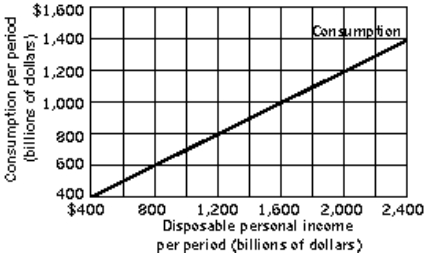 -Refer to Figure 13-1.If disposable personal income is $400 billion, what is the amount of personal saving?
(Multiple Choice)
4.8/5 (36)
In a graph with real GDP on the horizontal axis and aggregate expenditures on the vertical axis, induced aggregate expenditures are represented by
(Multiple Choice)
4.9/5 (33)
If an economy spends 90% of any increase in real GDP, then an increase in autonomous investment of $1 billion would result ultimately in an increase in equilibrium real GDP of
(Multiple Choice)
4.7/5 (35)
Figure 13-4
-Refer to Figure 13-4.Let Y = real GDP, AE = Aggregate Expenditures, C = Consumption,
IP = Planned Investment.Suppose AE = C + IP, and IP is autonomous.If the level of real GDP equals $5,000 billion, and if there are no changes in the consumption function or in planned investment, then we can expect that, in the next period, real GDP will
(Multiple Choice)
4.8/5 (44)
If consumption is $80 billion when income is $100, the most likely value for the marginal propensity to consume is 0.8.
(True/False)
4.8/5 (42)
Filters
- Essay(0)
- Multiple Choice(0)
- Short Answer(0)
- True False(0)
- Matching(0)