Deck 13: Asking and Answering Questions About the Difference Between Two Means
Full screen (f)
Question
The data below give the weights in ounces of randomly-selected bars of bath soap produced by two different molding machines. 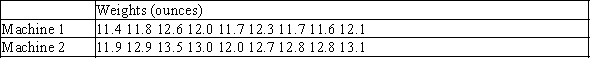 The question of interest is whether these two molding machines produce soap bars of differing average weight. Find a 95% confidence interval for the population difference assuming that the weights for the two machines are approximately normal.
A)(-1.760, -0.091)
B)(-1.200, -0.464)
C)(-0.354, 0.173)
D)(-1.280, -0.384)
The question of interest is whether these two molding machines produce soap bars of differing average weight. Find a 95% confidence interval for the population difference assuming that the weights for the two machines are approximately normal.A)(-1.760, -0.091)
B)(-1.200, -0.464)
C)(-0.354, 0.173)
D)(-1.280, -0.384)
Question
When testing hypotheses about and constructing confidence intervals for μ1 − μ2, we utilize the statistic,  . What are the mean and standard deviation of the sampling distribution of
  ?
?
. What are the mean and standard deviation of the sampling distribution of ? Question
Karl is a software developer who is interested in determining whether two random number generators have the same population mean.Random number generator A has a population standard deviation of 1.00 and random number generator B has a population standard deviation of 1.25.
Karl took a sample of 10 trials from each generator.The results are summarized below.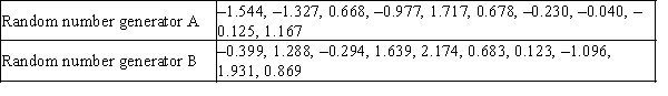 Find the P-value for the test of the difference between the population means for these two generators.
A)0.171
B)0.169
C)0.086
D)0.095
Karl took a sample of 10 trials from each generator.The results are summarized below.
Find the P-value for the test of the difference between the population means for these two generators.A)0.171
B)0.169
C)0.086
D)0.095
Question
Body fat and lean body mass can be estimated in living animals by measuring the total body electrical conductivity (TOBEC). This technique is useful when attempting to determine if "diet drugs" are working on laboratory rats over time--the researchers need not sacrifice the animals to measure the amount of adipose body fat after periods of drug usage. However, the procedure requires that the animal be totally inside the measurement chamber, which is fairly small. Some rats are so big their tails must be tucked under their bodies before putting them into the measurement chamber. This is causing concern among the researchers, because there is a possibility the tail position might alter the measurements. To see if the TOBEC measurement is altered by the tail position of the rats, an experiment was run on 16 rats ranging in weight from 210 to 505g.
The rats were randomly assigned the order of measurement, with 8 rats measured in the tail-under position first, and 8 rats in the tail-extended position.The data for the lean mass measures, and the differences, are presented in the table below.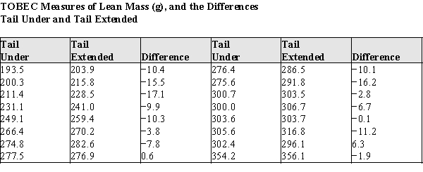
a)Using graphical display(s) of your choice show that the assumptions necessary for the paired t-test are plausible.
b)Test the hypothesis that there is no difference between the population mean TOBEC measurements of rats in the tail-under vs.the tail-extended positions.For purposes of the statistics you may assume that these rats are a random sample of laboratory rats.
c)Write a short paragraph based on your analysis above, explaining your results for laboratory technicians.Your paragraph should advise them whether or not it is necessary to make sure the tail positions of the rats are the same when replicating the lean mass body measurements during the experiment.
Question
For two independent samples, 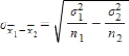 .
.
. Question
A researcher investigates the effect of a new drug on resting heart rate.The resting heart rates of 15 patients are measured before and after administration of the drug. The results are summarized in the table below. 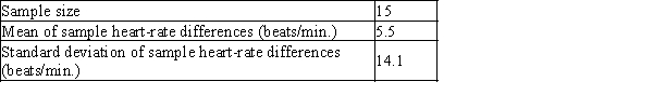 The question of interest is whether the resting heart rate increases after administration of the drug. Find the 95% confidence interval for the mean between population differences for heart rates.
A)(-2.64, 13.64))
B)(-3.64, 14.64)
C)(-2.31.13.31)
D)(-1.64, 12.64)
The question of interest is whether the resting heart rate increases after administration of the drug. Find the 95% confidence interval for the mean between population differences for heart rates.A)(-2.64, 13.64))
B)(-3.64, 14.64)
C)(-2.31.13.31)
D)(-1.64, 12.64)
Question
Samples from two independent, normally-distributed populations produced the following results. 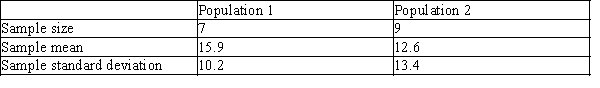 Calculate the 95% confidence interval for the difference between population means, µ1-µ2
A)(-9.65, 15.65)
B)(-8.26, 14.86)
C)(-10.10, 16.74)
D)(-0.55, 2.54)
Calculate the 95% confidence interval for the difference between population means, µ1-µ2A)(-9.65, 15.65)
B)(-8.26, 14.86)
C)(-10.10, 16.74)
D)(-0.55, 2.54)
Question
The data below give the weights in ounces of randomly-selected bars of bath soap produced by two different molding machines. 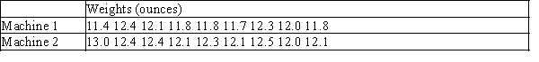 The question of interest is whether these two molding machines produce soap bars of differing average weight. Find the P-value for the this test assuming that the weights for the two machines are approximately normal..
A)0.014
B)0.311
C)0.038
D)0.054
The question of interest is whether these two molding machines produce soap bars of differing average weight. Find the P-value for the this test assuming that the weights for the two machines are approximately normal..A)0.014
B)0.311
C)0.038
D)0.054
Question
Question
Researchers have hypothesized that female Downy Woodpeckers avoid the feeding areas of socially dominant males; that is, the males chase them away from prime spots. An alternative opinion is that there are important physical characteristics of males and females that might lead them to choose different foraging locations. One such characteristic could be the bill length of the males and females; it may be that longer bills let one gender or the other drill deeper into a tree and thus get more food per tree.
The data in the table below are the bill lengths of 12 male and 12 female randomly selected Downy Woodpeckers caught and released in a banding survey. The investigators would like to know whether these data provide evidence that the males and females differ in bill size.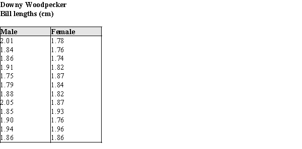
a)Using a graphical display of your choosing, assess the plausibility of the assumption that the distributions of bill lengths are approximately normal. State your conclusion in a few sentences.
b)Assuming that it is OK to proceed with a two-sample t procedure, determine if there is sufficient evidence to conclude that there is a difference in mean bill length for males and females.
c)In a few sentences, state any concerns you have about your conclusions in part (b), based on your results from part (a). If you have no concerns, write "No concerns."
Question
Question
Samples from two independent, normally-distributed populations produced the following results. 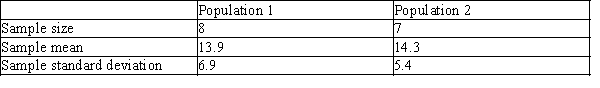 Calculate the test statistic for the difference between population means, µ1-µ2
A)-0.123
B)-0.126
C)-0.107
D)-0.058
Calculate the test statistic for the difference between population means, µ1-µ2A)-0.123
B)-0.126
C)-0.107
D)-0.058
Question
Question
Question
Does the gas leakage rate from automobile tires depend on the type of gas used to fill them? A sample of automobile tires are filled with nitrogen to a pressure of 1 atmosphere, and the time is measured for the internal pressure to fall to 0.9 atmospheres. The experiment is repeated for this sample of tires, but using sulfur hexafluoride in place of nitrogen. The results are summarized below. 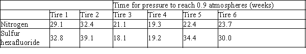 The null hypothesis is that the difference in mean population leak times is zero. Calculate a 95% confidence interval for the mean of population differences in leak times. Assume the leak times are normally distributed.
A)(-5.07, -3.47)
B)(-8.65, 0.12)
C)(-9.86, 1.33)
D)(-9.15, 0.61)
The null hypothesis is that the difference in mean population leak times is zero. Calculate a 95% confidence interval for the mean of population differences in leak times. Assume the leak times are normally distributed.A)(-5.07, -3.47)
B)(-8.65, 0.12)
C)(-9.86, 1.33)
D)(-9.15, 0.61)
Question
A researcher investigates the effect of a new drug on resting heart rate.The resting heart rates of 15 patients are measured before and after administration of the drug. The results are summarized in the table below.  The question of interest is whether the resting heart rate increases after administration of the drug. Find the value of the test statistic.
A)5.5
B)5.67
C)0.39
D)1.51
The question of interest is whether the resting heart rate increases after administration of the drug. Find the value of the test statistic.A)5.5
B)5.67
C)0.39
D)1.51
Question
Samples from two independent, normally-distributed populations produced the following results. 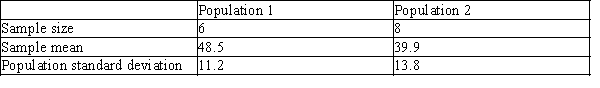 Calculate the test statistic for the difference between population means,
  .
.
A)1.889
B)8.6
C)1.128
D)1.286
Calculate the test statistic for the difference between population means, .A)1.889
B)8.6
C)1.128
D)1.286
Question
Does the gas leakage rate from automobile tires depend on the type of gas used to fill them?
A sample of automobile tires are filled with nitrogen to a pressure of 1 atmosphere, and the time is measured for the internal pressure to fall to 0.9 atmospheres. The experiment is repeated for this sample of tires, but using sulfur hexafluoride in place of nitrogen. The results are summarized below.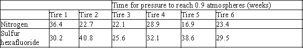 The null hypothesis is that the difference in mean population leak times is zero. Find the P-value for this test. Assume that the leakage times are normally distributed.
A)0.084
B)0.133
C)0.127
D)0.168
A sample of automobile tires are filled with nitrogen to a pressure of 1 atmosphere, and the time is measured for the internal pressure to fall to 0.9 atmospheres. The experiment is repeated for this sample of tires, but using sulfur hexafluoride in place of nitrogen. The results are summarized below.
The null hypothesis is that the difference in mean population leak times is zero. Find the P-value for this test. Assume that the leakage times are normally distributed.A)0.084
B)0.133
C)0.127
D)0.168
Question
When testing hypotheses about and constructing confidence intervals for μ1 − μ2, we utilize the statistic,  . What are the mean and variance of the sampling distribution of
  ?
?
. What are the mean and variance of the sampling distribution of ? Question
Question
As part of the foraging behavior assessment described in the previous problem, investigators also measured the bill depths of the male and female Downy Woodpeckers. Summary statistics for these measures are given in the table below: 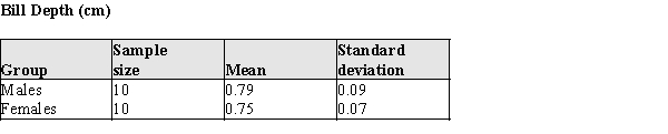 An initial analysis of the data revealed that it was reasonable to assume the bill depths for both sexes are approximately normal.
a)Construct a 95% confidence interval for the difference in bill depths of the males and females.
b)Do the data indicate that the bill depths differ? Justify your answer statistically.
An initial analysis of the data revealed that it was reasonable to assume the bill depths for both sexes are approximately normal.a)Construct a 95% confidence interval for the difference in bill depths of the males and females.
b)Do the data indicate that the bill depths differ? Justify your answer statistically.
Question
In 1992 Hurricane Andrew struck Florida causing widespread devastation. The eye of Hurricane Andrew passed directly over a site where scientists were studying the ecology of white-tailed deer. The deer had been radio-collared prior to Andrew's appearance, and the hurricane provided an opportunity to study the effects of an awesome storm on the deer. The investigators felt that the home ranges of the deer would change, but were unsure of the direction of the change. (The home range is the average area an animal occupies while foraging for food and defending its territory.) Home ranges of animals usually do not change much unless an area is under ecological stress.
The home range data for a random sample of 18 white-tailed radio-collared deer are shown below in Table 1. The raw area of the home range for each of the deer is reported in hectares for the pre-hurricane year of 1992 and the post hurricane year of 1993. (A hectare is a metric unit of area equal to 2.471 acres.)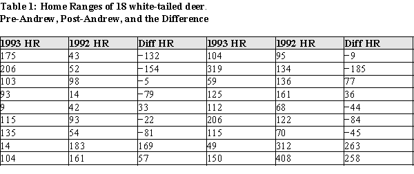
a)Using graphical display(s) of your choice show that the assumptions necessary for determining any change in the mean home ranges are plausible.
b)Construct a 95% confidence interval for the difference in means of the home ranges from before Andrew to after Andrew.
c)Do the data provide evidence of a change in the size of the home ranges after Hurricane Andrew? Provide statistical justification for your response.
Question
The home range of an animal is the average area an animal occupies while foraging for food and defending its territory. It is thought that home ranges of animals usually do not change much, except when an area is under ecological stress. As part of a study of white-tailed deer in Florida in 1991 and 1992, deer were radiocollared and their movements followed over the course of a year. The home range data for a random sample of 18 white-tailed deer are shown below in Table 1. The raw area of the home range for each of the deer is reported in hectares for the years 1991 and 1992. (A hectare is a metric unit of area equal to 2.471 acres.) The investigators are interested in determining whether the home range white-tailed deer change over the course of as little time as a year. 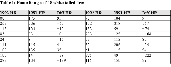
a)Using graphical display(s) of your choice show that the assumptions necessary for determining a change in the mean home ranges are plausible.
b)Construct a 95% confidence interval for the difference in means of the home ranges from 1991 to 1992.
c)Do the data provide evidence of a change in the size of the home ranges between 1991 and 1992? Provide statistical justification for y.
Question
A recent paper described an experiment in which 72 students at a university were assigned at random to one of two groups. All students took a class from the same instructor in the same semester. Students were required to report to an assigned room at a set time to fill out a course evaluation. One group of students reported to a room where they were offered a small bar of chocolate as they entered. The other group reported to a different room where they were not offered chocolate. Summary statistics for the overall course evaluation score are given in the accompanying table. 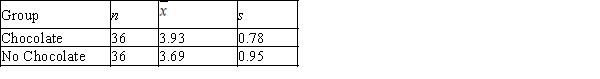 A 95% confidence interval for the mean difference in overall course evaluation score is:
A)
B)
C)
D)
E)
A 95% confidence interval for the mean difference in overall course evaluation score is:A)
B)
C)
D)
E)
Question
Question
In a recent paper, the authors distinguish between spending money on experiences (such as travel) and spending money on material possessions (such as a car). In an experiment to determine if the type of purchase affects how happy people are after the purchase has been made, 155 college students were randomly assigned to one of two groups. The students in the "experiential" group were asked to recall a time when they spent about $250 on an experience. They rated this purchase on three different happiness scales that were then combined into an overall measure of happiness. The students assigned to the "material" group recalled a time that they spent about $250 on an object and rated this purchase in the same manner. The mean happiness score was 5.62 for the experiential group and 5.44 for the material group.
Which of the following hypotheses should be tested to determine the author conclusion that, on average, "experiential purchases induced more reported happiness"?
A)
B)
C)
D)
E)
Which of the following hypotheses should be tested to determine the author conclusion that, on average, "experiential purchases induced more reported happiness"?
A)
B)
C)
D)
E)
Question
Researchers want to check whether women really speak more than men per day. During the day conversations of 873 adults selected randomly were recorded and then analyzed for the number of words. Researchers report that the mean number of words per day for the sample of women was 15,734 and the mean number for the sample of men was 13,813. The resulting data are given in the accompanying table.
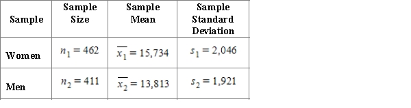
Construct and interpret a 95% confidence interval estimate for the difference in mean number of words per day for women and men.
A)The confidence interval is (1,700;2,142) You can be 95% confident that the actual difference in mean number of words per day for women and men is between 1,700 and 2,142
B)The confidence interval is (1,574;2,268) You can be 95% confident that the actual difference in mean number of words per day for women and men is between 1,574 and 2,268.
C)The confidence interval is (1,657;2,185) You can be 95% confident that the actual difference in mean number of words per day for women and men is between 1,657 and 2,185.
D) The confidence interval is (1,787;2,055) You can be 95% confident that the actual difference in mean number of words per day for women and men is between 1,787 and 2,055.
E)The confidence interval is (1,915;1,927) You can be 95% confident that the actual difference in mean number of words per day for women and men is between 1,915 and 1,927.
Question
Researchers assessed the effectiveness of courses on logic and computer thinking for adult residents of the city. 10 adults were tested on the topic of logic and computer thinking before and after the courses, their knowledge was evaluated on a scale of 0 to 20. The resulting data are given in the accompanying table. Assume that the sample of 10 adults is representative of adult residents of the city. 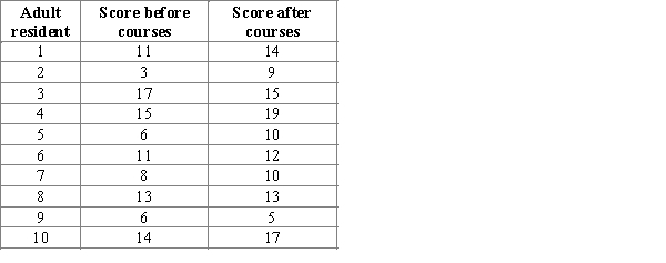 Construct and interpret a 90% confidence interval estimate for the difference in the mean score before and after courses on logic and computer thinking.
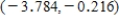
A)The confidence interval is
 .
.
You can be 90% confident that the actual difference in the mean score before and after courses on logic and computer thinking for adult residents of the city is between -3.784 and -0.216.
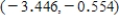
B)The confidence interval is
 .
.
You can be 90% confident that the actual difference in the mean score before and after courses on logic and computer thinking for adult residents of the city is between -3.446 and -0.554.
C)The confidence interval is
 .
.
You can be 90% confident that the actual difference in the mean score before and after courses on logic and computer thinking for adult residents of the city is between -4.564 and 0.564.
D)The confidence interval is
 .
.
You can be 90% confident that the actual difference in the mean score before and after courses on logic and computer thinking for adult residents of the city is between -6.573 and 2.573.
E)The confidence interval is
 .
.
You can be 90% confident that the actual difference in the mean score before and after courses on logic and computer thinking for adult residents of the city is between -1.446 and 1.446.
Construct and interpret a 90% confidence interval estimate for the difference in the mean score before and after courses on logic and computer thinking.A)The confidence interval is
.You can be 90% confident that the actual difference in the mean score before and after courses on logic and computer thinking for adult residents of the city is between -3.784 and -0.216.
B)The confidence interval is
.You can be 90% confident that the actual difference in the mean score before and after courses on logic and computer thinking for adult residents of the city is between -3.446 and -0.554.
C)The confidence interval is
.You can be 90% confident that the actual difference in the mean score before and after courses on logic and computer thinking for adult residents of the city is between -4.564 and 0.564.
D)The confidence interval is
.You can be 90% confident that the actual difference in the mean score before and after courses on logic and computer thinking for adult residents of the city is between -6.573 and 2.573.
E)The confidence interval is
.You can be 90% confident that the actual difference in the mean score before and after courses on logic and computer thinking for adult residents of the city is between -1.446 and 1.446.
Question
Suppose 9 adult smokers were randomly selected. Researchers want to check whether the movie about the dangers of smoking affects the number of cigarettes smoked. The number of cigarettes per day before and after watching the movie was recorded for each smoker from the sample and resulting data are given in the accompanying table. 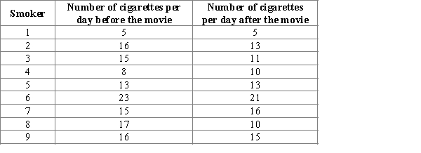 Select the most appropriate 95% bootstrap confidence interval for a difference in the mean number of cigarettes per day before and after watching the movie for adult smokers and its correct interpretation.
A)The bootstrap confidence interval is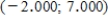 .You can be 95% confident that the actual difference in mean number of cigarettes per day before and after watching the movie is between -2.000 and 7.000.
B)The bootstrap confidence interval is .You can be 95% confident that the actual difference in mean number of cigarettes per day before and after watching the movie is between 0.222 and 3.000.
C)The bootstrap confidence interval is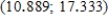 .You can be 95% confident that the actual difference in mean number of cigarettes per day before and after watching the movie is between 10.889 and 17.333.
D)The bootstrap confidence interval is .You can be 95% confident that the actual difference in mean number of cigarettes per day before and after watching the movie is between 0.000 and 3.333.
E)The bootstrap confidence interval is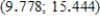 .You can be 95% confident that the actual difference in mean number of cigarettes per day before and after watching the movie is between 9.778 and 15.444.
Select the most appropriate 95% bootstrap confidence interval for a difference in the mean number of cigarettes per day before and after watching the movie for adult smokers and its correct interpretation.A)The bootstrap confidence interval is
.You can be 95% confident that the actual difference in mean number of cigarettes per day before and after watching the movie is between -2.000 and 7.000.B)The bootstrap confidence interval is
.You can be 95% confident that the actual difference in mean number of cigarettes per day before and after watching the movie is between 0.222 and 3.000.C)The bootstrap confidence interval is
.You can be 95% confident that the actual difference in mean number of cigarettes per day before and after watching the movie is between 10.889 and 17.333.D)The bootstrap confidence interval is
.You can be 95% confident that the actual difference in mean number of cigarettes per day before and after watching the movie is between 0.000 and 3.333.E)The bootstrap confidence interval is
.You can be 95% confident that the actual difference in mean number of cigarettes per day before and after watching the movie is between 9.778 and 15.444. Question
Suppose 8 adult patients with the same diagnosis were randomly selected. Researchers want to check whether the injected medication will affect the change in body temperature. The patient's body temperature was measured before and after the injected medication and resulting data are given in the accompanying table. 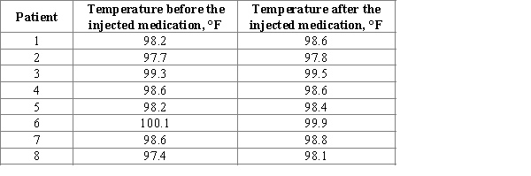 Construct and interpret a 95% confidence interval estimate for the difference in mean temperature before and after the injected medication.
A)The confidence interval is
 .
.
You can be 95% confident that the actual difference in mean temperature before and after the injected medication for adult patients with this diagnosis is between -0.379 and -0.021.
B)The confidence interval is
 .
.
You can be 95% confident that the actual difference in mean temperature before and after the injected medication for adult patients with this diagnosis is between -0.832 and 0.432.
C)The confidence interval is
 .
.
You can be 95% confident that the actual difference in mean temperature before and after the injected medication for adult patients with this diagnosis is between -0.423 and 0.023.
D)The confidence interval is
 .
.
You can be 95% confident that the actual difference in mean temperature before and after the injected medication for adult patients with this diagnosis is between -0.223 and 0.223.
E)The confidence interval is
 .
.
You can be 95% confident that the actual difference in mean temperature before and after the injected medication for adult patients with this diagnosis is between -0.531 and 0.131.
Construct and interpret a 95% confidence interval estimate for the difference in mean temperature before and after the injected medication.A)The confidence interval is
.You can be 95% confident that the actual difference in mean temperature before and after the injected medication for adult patients with this diagnosis is between -0.379 and -0.021.
B)The confidence interval is
.You can be 95% confident that the actual difference in mean temperature before and after the injected medication for adult patients with this diagnosis is between -0.832 and 0.432.
C)The confidence interval is
.You can be 95% confident that the actual difference in mean temperature before and after the injected medication for adult patients with this diagnosis is between -0.423 and 0.023.
D)The confidence interval is
.You can be 95% confident that the actual difference in mean temperature before and after the injected medication for adult patients with this diagnosis is between -0.223 and 0.223.
E)The confidence interval is
.You can be 95% confident that the actual difference in mean temperature before and after the injected medication for adult patients with this diagnosis is between -0.531 and 0.131.
Question
Question
When a surgeon repairs injuries, sutures (stitched knots) are sometimes used to hold together and stabilize the injured area. If these knots elongate and loosen, the injury may not heal properly. Researchers at the University of California, San Francisco, tied a particular type of knot with two types of suture material, Maxon and Ticron. Suppose that 112 tissue specimens were available and that for each specimen the type of suture material was randomly assigned. The investigators tested the knots to see how much they elongated. For purposes of this exercise, you can assume that it is reasonable to regard the elongation distributions as approximately normal. Which of the following hypotheses should be tested to determine if there is a significant difference in mean elongation between Maxon versus Ticron threads?
A)
B)
C)
D)
E)
A)
B)
C)
D)
E)
Question
The Iowa Tests of Basic Skills is a collection of various achievement tests given to students in grades 1 - 8. Student achievement levels are reported on a scale that runs from 0 to 13. The North Snowshoe Community Schools are evaluating their reading program for students whose native language is not English. In one part of the study the reading comprehension of 10 students, randomly selected from a large population of students in the program, take the Reading Comprehension test in third and fourth grade. Their scores for each year, in grade equivalents, are listed below. 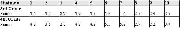 "Normal" growth, by definition, is a change of 1.0. Using the data above, test the hypothesis that the difference in means for 3rd and 4th grade students in this program for non-native English speakers is equal to 1.0.
"Normal" growth, by definition, is a change of 1.0. Using the data above, test the hypothesis that the difference in means for 3rd and 4th grade students in this program for non-native English speakers is equal to 1.0. Question
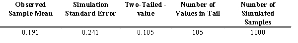
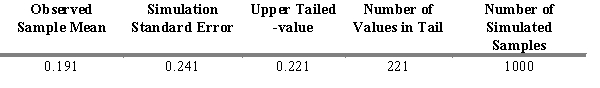
The researchers suggested that the time of the second race in karting is less than during the first race because a person remembers the track. Suppose 8 adults were randomly selected. The time spent on the first and second race was recorded for each person from the sample and resulting data are given in the accompanying table. 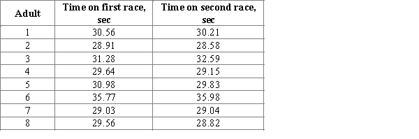 Do these data support the claim that the mean difference in time spent on the first and second race is greater than zero? Use a randomization test to select the appropriate output for one set of 1000 simulated sample differences in means and carry out a hypothesis test for a difference in means.
A)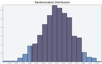
 Since the approximate P-value is greater than
  , we reject H0 for a significance level of 0.05.So the sample provides convincing evidence that the mean difference in time spent on the first and second race is greater than zero.
B)
 Since the approximate P-value is greater than
  , we reject H0 for a significance level of 0.05.So the sample provides convincing evidence that the mean difference in time spent on the first and second race is greater than zero.
C)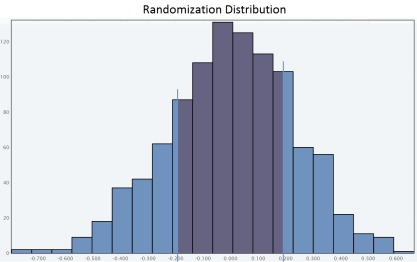
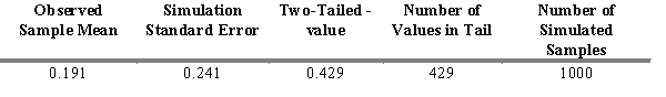
Since the approximate P-value is greater than , we fail to reject H0 for a significance level of 0.05.So the sample does not provide convincing evidence that the mean difference in time spent on the first and second race is greater than zero.
D)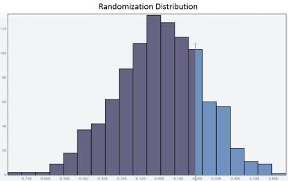

Since the approximate P-value is greater than , we fail to reject H0 for a significance level of 0.05.So the sample does not provide convincing evidence that the mean difference in time spent on the first and second race is greater than zero.
E)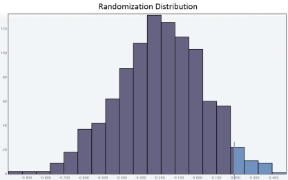

Since the approximate P-value is less than , we reject H0 for a significance level of 0.05.So the sample provides convincing evidence that the mean difference in time spent on the first and second race is greater than zero.
Do these data support the claim that the mean difference in time spent on the first and second race is greater than zero? Use a randomization test to select the appropriate output for one set of 1000 simulated sample differences in means and carry out a hypothesis test for a difference in means.A)
Since the approximate P-value is greater than , we reject H0 for a significance level of 0.05.So the sample provides convincing evidence that the mean difference in time spent on the first and second race is greater than zero.B)
Since the approximate P-value is greater than , we reject H0 for a significance level of 0.05.So the sample provides convincing evidence that the mean difference in time spent on the first and second race is greater than zero.C)
Since the approximate P-value is greater than
, we fail to reject H0 for a significance level of 0.05.So the sample does not provide convincing evidence that the mean difference in time spent on the first and second race is greater than zero.D)
Since the approximate P-value is greater than
, we fail to reject H0 for a significance level of 0.05.So the sample does not provide convincing evidence that the mean difference in time spent on the first and second race is greater than zero.E)
Since the approximate P-value is less than
, we reject H0 for a significance level of 0.05.So the sample provides convincing evidence that the mean difference in time spent on the first and second race is greater than zero. Question
A common memory task is the classification of objects into categories. For example, a table is a piece of furniture; a dog is an animal, etc. This classification capability was used in a recent study of divided attention. College Psychology students were randomly selected and randomly assigned to one of two experimental conditions: divided attention and no divided attention. Students in the "divided attention" group were asked to memorize a list of 36 words while simultaneously listening to a tape recorder; students in a control group were told to memorize a list of 36 words and did not listen to a tape recorder. Each student was then asked to classify the 36 words into 6 categories. (There were 6 words in each category.) The distributions of the correct number of recalled words / category were approximately normal in each of the groups, and a summary of the data for the words/category recalled are presented below: 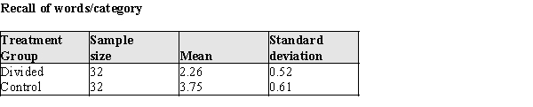
a)Is there evidence that the memory performance differs in the two groups? Test the appropriate hypothesis using α = 0.05.
b)One possible implication of this study is that high school students should not be dividing their attention by listening to music while studying. What results, if any, of this study would support the contention that students should not be dividing their attention?
Question
Viruses are infectious agents that often cause diseases in plants. Different viruses have different potency levels, and this fact can be used to detect whether a new virus is infecting plants in the field. In a potency comparison experiment, two viruses were placed on a tobacco leaf of 10 randomly selected tobacco plants in a field. The viruses were randomly assigned to one-half of each of the leaves. The table below presents the potency of the viruses, as measured by the number of lesions appearing on the leaf half. 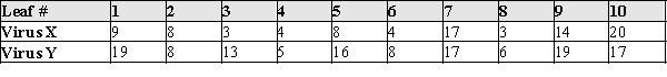 Test the hypothesis that there is no difference in mean number of lesions for Virus X and Virus Y.
Test the hypothesis that there is no difference in mean number of lesions for Virus X and Virus Y. Question
An article describes a study of the effectiveness of a fabric device that acts like a support stocking for a weak or damaged heart. In the study, 94 people who consented to treatment were assigned at random to either a standard treatment (S) consisting of drugs or the experimental treatment (E) that consisted of drugs plus surgery to install the stocking. After two years, 36% of the 61 patients receiving the stocking had improved,while 23% of the patients receiving the standard treatment had improved. Which of the following hypotheses should be tested to determine whether the proportion of patients who improve is significantly higher for the experimental treatment than for the standard treatment?
A)
B)
C)
D)
E)
A)
B)
C)
D)
E)
Question
Body fat and lean body mass can be estimated in living animals by measuring the total body electrical conductivity (TOBEC). This technique is useful when attempting to determine if "diet drugs" are working on laboratory rats over time--the researchers need not sacrifice the animals to measure the amount of adipose body fat after periods of drug usage. However, the procedure requires that the animal be totally inside the measurement chamber, which is fairly small. Some rats are so big that their tails must be tucked under their bodies before putting them into the measurement chamber. This is causing concern among the researchers, because there is a possibility the tail position might alter the measurements. To see if the TOBEC measurement is altered by the tail position of the rats, an experiment was run on 16 rats ranging in weight from 210 to 505
g.The rats were randomly assigned the order of measurement, with 8 rats measured in the tail-under position first, and 8 rats in the tail-extended position.The data for the body fat measures, and the differences, are presented in the table below.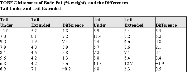 a)Using graphical display(s) of your choice show that the assumptions necessary for the paired t-test are plausible.b)Test the hypothesis that there is no difference between the population mean TOBEC body fat measurements of rats in the tail-under vs.the tail-extended positions.For purposes of the statistics you may assume that these rats are a random sample of laboratory rats.c)Write a short paragraph based on your analysis above, explaining your results for laboratory technicians.Your paragraph should advise them whether or not it is necessary to make sure the tail positions of the rats are the same when replicating the lean mass body measurements during the experiment.
g.The rats were randomly assigned the order of measurement, with 8 rats measured in the tail-under position first, and 8 rats in the tail-extended position.The data for the body fat measures, and the differences, are presented in the table below.
a)Using graphical display(s) of your choice show that the assumptions necessary for the paired t-test are plausible.b)Test the hypothesis that there is no difference between the population mean TOBEC body fat measurements of rats in the tail-under vs.the tail-extended positions.For purposes of the statistics you may assume that these rats are a random sample of laboratory rats.c)Write a short paragraph based on your analysis above, explaining your results for laboratory technicians.Your paragraph should advise them whether or not it is necessary to make sure the tail positions of the rats are the same when replicating the lean mass body measurements during the experiment. Question
The perception of danger is an important characteristic for survival of animals. In a field experiment in Costa Rica, investigators located and directly approached black iguanas; that is, they walked straight towards them. Two treatments were randomly assigned to the individual iguanas. In one treatment the investigator gazed at the iguana while approaching, "maintaining eye contact." In a second treatment, the investigator did not gaze at the iguana while approaching. The outcome measure was the distance of the investigator from the iguana when it decided to run away. The researchers believe that eye contact is noticed by the iguana, leading to a longer approach distance. Data from this experiment appears in the table below. 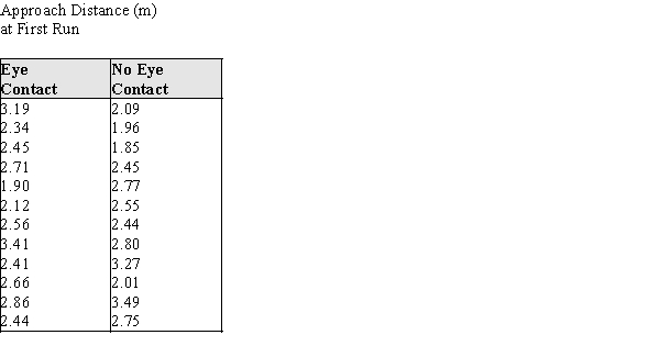
a)Using a graphical display of your choosing, assess the assumption that the distributions of approach distances are approximately normal. State your conclusion in a few sentences.
b)Assuming that it is OK to proceed with a two-sample t procedure, determine if there is sufficient evidence to conclude that there is a shorter mean approach distance for the "Eye contact" group.
c)In a few sentences, state any concerns you have about your conclusions in part (b), based on your results from part (a). If you have no concerns, write "No concerns."
Question
A study is conducted to determine the effect of different doses of a cold medication on reaction times. In a study of 20 participants between 20 and 25 years of age, half were given a single dose of medication and the other half were given two doses. Thirty minutes after dosing, a simple mechanical experiment measured subject reaction time in milliseconds. The results are summarized below. 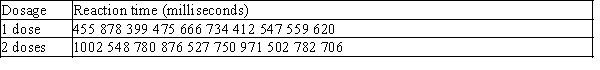 Calculate the 95% confidence interval for the difference in reaction times for these two groups. Assume that the reaction times are normally-distributed and that the treatments were randomly assigned.
A)(-351, 12)
B)(-326, -14)
C)(-385, 46)
D)(-201, -28)
Calculate the 95% confidence interval for the difference in reaction times for these two groups. Assume that the reaction times are normally-distributed and that the treatments were randomly assigned.A)(-351, 12)
B)(-326, -14)
C)(-385, 46)
D)(-201, -28)
Question
As part of the iguana risk assessment experiment described in the previous problem, investigators replicated the experiment with one difference--the investigators approached the iguanas at a tangent, passing by the iguana with a closest distance being 2 meters. Summary statistics for the approach distances for the two treatments, Eye Contact and No Eye Contact, are given in the table below: 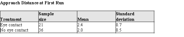 An initial analysis of the data revealed that it was reasonable to assume the population approach distances at first run were both approximately normal.
a)Construct a 95% confidence interval for the difference in approach distances for the eye contact and no eye contact treatments.
b)Do the data indicate that for a tangential approach, the population means differ? Justify your answer statistically.
An initial analysis of the data revealed that it was reasonable to assume the population approach distances at first run were both approximately normal.a)Construct a 95% confidence interval for the difference in approach distances for the eye contact and no eye contact treatments.
b)Do the data indicate that for a tangential approach, the population means differ? Justify your answer statistically.
Question
A common memory task is the classification of objects into categories. For example, a table is a piece of furniture; a dog is an animal, etc. This classification capability was used in a recent study of divided attention. Elderly adults were randomly selected from those answering a newspaper advertisement, and randomly assigned to two conditions: divided attention and no divided attention. Subjects in the "divided attention" group were told to memorize a list of 36 words while simultaneously listening to a tape recorder; subjects in a control group were told to memorize a list of 36 words and did not listen to a tape recorder. Subjects were then asked to classify the 36 words into 6 categories. (There were 6 words in each category.) The distributions of the correct number of recalled words / category were approximately normal in each of the groups, and a summary of the data for the words/category recalled are presented below: 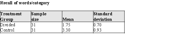
a)Is there evidence that the memory performance differs in the two groups? Test the appropriate hypothesis using α = .05.
b)One possible implication of this study is that high school students should not be dividing their attention by listening to music while studying. What results, if any, of this study would support the contention that students should not be dividing their attention?
Question
Question
Suppose a researcher is testing a new diet drug. She would like to determine if the drug helps to significantly increase weight loss versus a placebo. She randomly assigns 40 participants to the treatment group and 35 to the placebo group. After 4 weeks on identical diets, the mean weights loss (in pounds) for each group is computed. Results of the study are as follows:
Treatment Group
Placebo Group
n = 40
n = 35
 = 5.6
= 5.6
 = 1.6
= 1.6
s = 2.85
s = 1.47
Create a 95% confidence interval for the difference of treatment effects.
Treatment Group
Placebo Group
n = 40
n = 35
= 5.6 = 1.6s = 2.85
s = 1.47
Create a 95% confidence interval for the difference of treatment effects.
Question
Question
Suppose a researcher is testing a new diet drug. She would like to determine if the drug helps to significantly increase weight loss versus a placebo. She randomly assigns 40 participants to the treatment group and 35 to the placebo group. After 4 weeks on identical diets, the mean weights loss (in pounds) for each group is computed. Results of the study are as follows:
Treatment Group
Placebo Group
n = 40
n = 35 = 5.6
= 5.6  = 1.6
= 1.6
s = 2.85
s = 1.47
Perform a hypothesis test to draw a conclusion from this study. Show all your work.
Treatment Group
Placebo Group
n = 40
n = 35
= 5.6 = 1.6s = 2.85
s = 1.47
Perform a hypothesis test to draw a conclusion from this study. Show all your work.

Unlock Deck
Sign up to unlock the cards in this deck!
Unlock Deck
Unlock Deck
1/46
Play
Full screen (f)
Deck 13: Asking and Answering Questions About the Difference Between Two Means
1
The data below give the weights in ounces of randomly-selected bars of bath soap produced by two different molding machines. The question of interest is whether these two molding machines produce soap bars of differing average weight. Find a 95% confidence interval for the population difference assuming that the weights for the two machines are approximately normal.
A)(-1.760, -0.091)
B)(-1.200, -0.464)
C)(-0.354, 0.173)
D)(-1.280, -0.384)
The question of interest is whether these two molding machines produce soap bars of differing average weight. Find a 95% confidence interval for the population difference assuming that the weights for the two machines are approximately normal.A)(-1.760, -0.091)
B)(-1.200, -0.464)
C)(-0.354, 0.173)
D)(-1.280, -0.384)
(-1.280, -0.384)
2
When testing hypotheses about and constructing confidence intervals for μ1 − μ2, we utilize the statistic, . What are the mean and standard deviation of the sampling distribution of ?
. What are the mean and standard deviation of the sampling distribution of ?The mean of the sampling distribution of  is
is 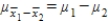 , the standard deviation is
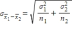 .
.
is , the standard deviation is . 3
Karl is a software developer who is interested in determining whether two random number generators have the same population mean.Random number generator A has a population standard deviation of 1.00 and random number generator B has a population standard deviation of 1.25.
Karl took a sample of 10 trials from each generator.The results are summarized below. Find the P-value for the test of the difference between the population means for these two generators.
A)0.171
B)0.169
C)0.086
D)0.095
Karl took a sample of 10 trials from each generator.The results are summarized below.
Find the P-value for the test of the difference between the population means for these two generators.A)0.171
B)0.169
C)0.086
D)0.095
0.171
4
Body fat and lean body mass can be estimated in living animals by measuring the total body electrical conductivity (TOBEC). This technique is useful when attempting to determine if "diet drugs" are working on laboratory rats over time--the researchers need not sacrifice the animals to measure the amount of adipose body fat after periods of drug usage. However, the procedure requires that the animal be totally inside the measurement chamber, which is fairly small. Some rats are so big their tails must be tucked under their bodies before putting them into the measurement chamber. This is causing concern among the researchers, because there is a possibility the tail position might alter the measurements. To see if the TOBEC measurement is altered by the tail position of the rats, an experiment was run on 16 rats ranging in weight from 210 to 505g.
The rats were randomly assigned the order of measurement, with 8 rats measured in the tail-under position first, and 8 rats in the tail-extended position.The data for the lean mass measures, and the differences, are presented in the table below.
a)Using graphical display(s) of your choice show that the assumptions necessary for the paired t-test are plausible.
b)Test the hypothesis that there is no difference between the population mean TOBEC measurements of rats in the tail-under vs.the tail-extended positions.For purposes of the statistics you may assume that these rats are a random sample of laboratory rats.
c)Write a short paragraph based on your analysis above, explaining your results for laboratory technicians.Your paragraph should advise them whether or not it is necessary to make sure the tail positions of the rats are the same when replicating the lean mass body measurements during the experiment.
The rats were randomly assigned the order of measurement, with 8 rats measured in the tail-under position first, and 8 rats in the tail-extended position.The data for the lean mass measures, and the differences, are presented in the table below.
a)Using graphical display(s) of your choice show that the assumptions necessary for the paired t-test are plausible.
b)Test the hypothesis that there is no difference between the population mean TOBEC measurements of rats in the tail-under vs.the tail-extended positions.For purposes of the statistics you may assume that these rats are a random sample of laboratory rats.
c)Write a short paragraph based on your analysis above, explaining your results for laboratory technicians.Your paragraph should advise them whether or not it is necessary to make sure the tail positions of the rats are the same when replicating the lean mass body measurements during the experiment.
Unlock Deck
Unlock for access to all 46 flashcards in this deck.
Unlock Deck
k this deck
5
For two independent samples, .
. Unlock Deck
Unlock for access to all 46 flashcards in this deck.
Unlock Deck
k this deck
6
A researcher investigates the effect of a new drug on resting heart rate.The resting heart rates of 15 patients are measured before and after administration of the drug. The results are summarized in the table below. The question of interest is whether the resting heart rate increases after administration of the drug. Find the 95% confidence interval for the mean between population differences for heart rates.
A)(-2.64, 13.64))
B)(-3.64, 14.64)
C)(-2.31.13.31)
D)(-1.64, 12.64)
The question of interest is whether the resting heart rate increases after administration of the drug. Find the 95% confidence interval for the mean between population differences for heart rates.A)(-2.64, 13.64))
B)(-3.64, 14.64)
C)(-2.31.13.31)
D)(-1.64, 12.64)
Unlock Deck
Unlock for access to all 46 flashcards in this deck.
Unlock Deck
k this deck
7
Samples from two independent, normally-distributed populations produced the following results. Calculate the 95% confidence interval for the difference between population means, µ1-µ2
A)(-9.65, 15.65)
B)(-8.26, 14.86)
C)(-10.10, 16.74)
D)(-0.55, 2.54)
Calculate the 95% confidence interval for the difference between population means, µ1-µ2A)(-9.65, 15.65)
B)(-8.26, 14.86)
C)(-10.10, 16.74)
D)(-0.55, 2.54)
Unlock Deck
Unlock for access to all 46 flashcards in this deck.
Unlock Deck
k this deck
8
The data below give the weights in ounces of randomly-selected bars of bath soap produced by two different molding machines. The question of interest is whether these two molding machines produce soap bars of differing average weight. Find the P-value for the this test assuming that the weights for the two machines are approximately normal..
A)0.014
B)0.311
C)0.038
D)0.054
The question of interest is whether these two molding machines produce soap bars of differing average weight. Find the P-value for the this test assuming that the weights for the two machines are approximately normal..A)0.014
B)0.311
C)0.038
D)0.054
Unlock Deck
Unlock for access to all 46 flashcards in this deck.
Unlock Deck
k this deck
9
The number of degrees of freedom used in the two-sample t test for independent samples are the same as the degrees of freedom used in the construction of a confidence interval for μ1 − μ2.
Unlock Deck
Unlock for access to all 46 flashcards in this deck.
Unlock Deck
k this deck
10
Researchers have hypothesized that female Downy Woodpeckers avoid the feeding areas of socially dominant males; that is, the males chase them away from prime spots. An alternative opinion is that there are important physical characteristics of males and females that might lead them to choose different foraging locations. One such characteristic could be the bill length of the males and females; it may be that longer bills let one gender or the other drill deeper into a tree and thus get more food per tree.
The data in the table below are the bill lengths of 12 male and 12 female randomly selected Downy Woodpeckers caught and released in a banding survey. The investigators would like to know whether these data provide evidence that the males and females differ in bill size.
a)Using a graphical display of your choosing, assess the plausibility of the assumption that the distributions of bill lengths are approximately normal. State your conclusion in a few sentences.
b)Assuming that it is OK to proceed with a two-sample t procedure, determine if there is sufficient evidence to conclude that there is a difference in mean bill length for males and females.
c)In a few sentences, state any concerns you have about your conclusions in part (b), based on your results from part (a). If you have no concerns, write "No concerns."
The data in the table below are the bill lengths of 12 male and 12 female randomly selected Downy Woodpeckers caught and released in a banding survey. The investigators would like to know whether these data provide evidence that the males and females differ in bill size.
a)Using a graphical display of your choosing, assess the plausibility of the assumption that the distributions of bill lengths are approximately normal. State your conclusion in a few sentences.
b)Assuming that it is OK to proceed with a two-sample t procedure, determine if there is sufficient evidence to conclude that there is a difference in mean bill length for males and females.
c)In a few sentences, state any concerns you have about your conclusions in part (b), based on your results from part (a). If you have no concerns, write "No concerns."
Unlock Deck
Unlock for access to all 46 flashcards in this deck.
Unlock Deck
k this deck
11
When testing a hypothesis concerning the difference of two independent population means, if the variance of the difference is estimated using the sample variances, the resulting test statistic has a Normal distribution.
Unlock Deck
Unlock for access to all 46 flashcards in this deck.
Unlock Deck
k this deck
12
Samples from two independent, normally-distributed populations produced the following results. Calculate the test statistic for the difference between population means, µ1-µ2
A)-0.123
B)-0.126
C)-0.107
D)-0.058
Calculate the test statistic for the difference between population means, µ1-µ2A)-0.123
B)-0.126
C)-0.107
D)-0.058
Unlock Deck
Unlock for access to all 46 flashcards in this deck.
Unlock Deck
k this deck
13
The number of degrees of freedom of the two-sample t test are the same as the degrees of freedom for the paired t test statistic.
Unlock Deck
Unlock for access to all 46 flashcards in this deck.
Unlock Deck
k this deck
14
Suppose a researcher is collecting data to compare the average amount of soda consumed daily by men and women. The researcher will ask participants to state the amount of soda they consumed on the previous day. The researcher would like to determine if differences exist in the amount of soda consumed between the genders. Should the researcher use a procedure for two independent samples or paired data?
Unlock Deck
Unlock for access to all 46 flashcards in this deck.
Unlock Deck
k this deck
15
Does the gas leakage rate from automobile tires depend on the type of gas used to fill them? A sample of automobile tires are filled with nitrogen to a pressure of 1 atmosphere, and the time is measured for the internal pressure to fall to 0.9 atmospheres. The experiment is repeated for this sample of tires, but using sulfur hexafluoride in place of nitrogen. The results are summarized below. The null hypothesis is that the difference in mean population leak times is zero. Calculate a 95% confidence interval for the mean of population differences in leak times. Assume the leak times are normally distributed.
A)(-5.07, -3.47)
B)(-8.65, 0.12)
C)(-9.86, 1.33)
D)(-9.15, 0.61)
The null hypothesis is that the difference in mean population leak times is zero. Calculate a 95% confidence interval for the mean of population differences in leak times. Assume the leak times are normally distributed.A)(-5.07, -3.47)
B)(-8.65, 0.12)
C)(-9.86, 1.33)
D)(-9.15, 0.61)
Unlock Deck
Unlock for access to all 46 flashcards in this deck.
Unlock Deck
k this deck
16
A researcher investigates the effect of a new drug on resting heart rate.The resting heart rates of 15 patients are measured before and after administration of the drug. The results are summarized in the table below. The question of interest is whether the resting heart rate increases after administration of the drug. Find the value of the test statistic.
A)5.5
B)5.67
C)0.39
D)1.51
The question of interest is whether the resting heart rate increases after administration of the drug. Find the value of the test statistic.A)5.5
B)5.67
C)0.39
D)1.51
Unlock Deck
Unlock for access to all 46 flashcards in this deck.
Unlock Deck
k this deck
17
Samples from two independent, normally-distributed populations produced the following results. Calculate the test statistic for the difference between population means, .
A)1.889
B)8.6
C)1.128
D)1.286
Calculate the test statistic for the difference between population means, .A)1.889
B)8.6
C)1.128
D)1.286
Unlock Deck
Unlock for access to all 46 flashcards in this deck.
Unlock Deck
k this deck
18
Does the gas leakage rate from automobile tires depend on the type of gas used to fill them?
A sample of automobile tires are filled with nitrogen to a pressure of 1 atmosphere, and the time is measured for the internal pressure to fall to 0.9 atmospheres. The experiment is repeated for this sample of tires, but using sulfur hexafluoride in place of nitrogen. The results are summarized below. The null hypothesis is that the difference in mean population leak times is zero. Find the P-value for this test. Assume that the leakage times are normally distributed.
A)0.084
B)0.133
C)0.127
D)0.168
A sample of automobile tires are filled with nitrogen to a pressure of 1 atmosphere, and the time is measured for the internal pressure to fall to 0.9 atmospheres. The experiment is repeated for this sample of tires, but using sulfur hexafluoride in place of nitrogen. The results are summarized below.
The null hypothesis is that the difference in mean population leak times is zero. Find the P-value for this test. Assume that the leakage times are normally distributed.A)0.084
B)0.133
C)0.127
D)0.168
Unlock Deck
Unlock for access to all 46 flashcards in this deck.
Unlock Deck
k this deck
19
When testing hypotheses about and constructing confidence intervals for μ1 − μ2, we utilize the statistic, . What are the mean and variance of the sampling distribution of ?
. What are the mean and variance of the sampling distribution of ? Unlock Deck
Unlock for access to all 46 flashcards in this deck.
Unlock Deck
k this deck
20
The large sample z test for μ1 − μ2 can be used as long as at least one of the two sample sizes, n1 and n2, is greater than or equal to 30.
Unlock Deck
Unlock for access to all 46 flashcards in this deck.
Unlock Deck
k this deck
21
As part of the foraging behavior assessment described in the previous problem, investigators also measured the bill depths of the male and female Downy Woodpeckers. Summary statistics for these measures are given in the table below: An initial analysis of the data revealed that it was reasonable to assume the bill depths for both sexes are approximately normal.
a)Construct a 95% confidence interval for the difference in bill depths of the males and females.
b)Do the data indicate that the bill depths differ? Justify your answer statistically.
An initial analysis of the data revealed that it was reasonable to assume the bill depths for both sexes are approximately normal.a)Construct a 95% confidence interval for the difference in bill depths of the males and females.
b)Do the data indicate that the bill depths differ? Justify your answer statistically.
Unlock Deck
Unlock for access to all 46 flashcards in this deck.
Unlock Deck
k this deck
22
In 1992 Hurricane Andrew struck Florida causing widespread devastation. The eye of Hurricane Andrew passed directly over a site where scientists were studying the ecology of white-tailed deer. The deer had been radio-collared prior to Andrew's appearance, and the hurricane provided an opportunity to study the effects of an awesome storm on the deer. The investigators felt that the home ranges of the deer would change, but were unsure of the direction of the change. (The home range is the average area an animal occupies while foraging for food and defending its territory.) Home ranges of animals usually do not change much unless an area is under ecological stress.
The home range data for a random sample of 18 white-tailed radio-collared deer are shown below in Table 1. The raw area of the home range for each of the deer is reported in hectares for the pre-hurricane year of 1992 and the post hurricane year of 1993. (A hectare is a metric unit of area equal to 2.471 acres.)
a)Using graphical display(s) of your choice show that the assumptions necessary for determining any change in the mean home ranges are plausible.
b)Construct a 95% confidence interval for the difference in means of the home ranges from before Andrew to after Andrew.
c)Do the data provide evidence of a change in the size of the home ranges after Hurricane Andrew? Provide statistical justification for your response.
The home range data for a random sample of 18 white-tailed radio-collared deer are shown below in Table 1. The raw area of the home range for each of the deer is reported in hectares for the pre-hurricane year of 1992 and the post hurricane year of 1993. (A hectare is a metric unit of area equal to 2.471 acres.)
a)Using graphical display(s) of your choice show that the assumptions necessary for determining any change in the mean home ranges are plausible.
b)Construct a 95% confidence interval for the difference in means of the home ranges from before Andrew to after Andrew.
c)Do the data provide evidence of a change in the size of the home ranges after Hurricane Andrew? Provide statistical justification for your response.
Unlock Deck
Unlock for access to all 46 flashcards in this deck.
Unlock Deck
k this deck
23
The home range of an animal is the average area an animal occupies while foraging for food and defending its territory. It is thought that home ranges of animals usually do not change much, except when an area is under ecological stress. As part of a study of white-tailed deer in Florida in 1991 and 1992, deer were radiocollared and their movements followed over the course of a year. The home range data for a random sample of 18 white-tailed deer are shown below in Table 1. The raw area of the home range for each of the deer is reported in hectares for the years 1991 and 1992. (A hectare is a metric unit of area equal to 2.471 acres.) The investigators are interested in determining whether the home range white-tailed deer change over the course of as little time as a year.
a)Using graphical display(s) of your choice show that the assumptions necessary for determining a change in the mean home ranges are plausible.
b)Construct a 95% confidence interval for the difference in means of the home ranges from 1991 to 1992.
c)Do the data provide evidence of a change in the size of the home ranges between 1991 and 1992? Provide statistical justification for y.
Unlock Deck
Unlock for access to all 46 flashcards in this deck.
Unlock Deck
k this deck
24
A recent paper described an experiment in which 72 students at a university were assigned at random to one of two groups. All students took a class from the same instructor in the same semester. Students were required to report to an assigned room at a set time to fill out a course evaluation. One group of students reported to a room where they were offered a small bar of chocolate as they entered. The other group reported to a different room where they were not offered chocolate. Summary statistics for the overall course evaluation score are given in the accompanying table. A 95% confidence interval for the mean difference in overall course evaluation score is:
A)
B)
C)
D)
E)
A 95% confidence interval for the mean difference in overall course evaluation score is:A)
B)
C)
D)
E)
Unlock Deck
Unlock for access to all 46 flashcards in this deck.
Unlock Deck
k this deck
25
Suppose that you wish to compare two treatments for preventing baldness in men. (The measure of baldness you will use is the mean number of healthy hair follicles per square cm.) In some circumstances, you may be able to randomly assign the treatments to the men, and in some circumstances, you may not be able to randomly assign the treatments to the men. Respond to the following questions in a few sentences.
a)If you are testing the hypothesis that the means are equal for the population, how would your statistical procedures differ, if at all, depending on whether you randomly assigned subjects to treatments or whether you merely observed differences in men who chose one treatment or the other?
b)How would your interpretation of the results differ, if at all, depending on whether you randomly assigned subjects to treatments or whether you merely observed differences in men who chose one treatment or the other?
Unlock Deck
Unlock for access to all 46 flashcards in this deck.
Unlock Deck
k this deck
26
In a recent paper, the authors distinguish between spending money on experiences (such as travel) and spending money on material possessions (such as a car). In an experiment to determine if the type of purchase affects how happy people are after the purchase has been made, 155 college students were randomly assigned to one of two groups. The students in the "experiential" group were asked to recall a time when they spent about $250 on an experience. They rated this purchase on three different happiness scales that were then combined into an overall measure of happiness. The students assigned to the "material" group recalled a time that they spent about $250 on an object and rated this purchase in the same manner. The mean happiness score was 5.62 for the experiential group and 5.44 for the material group.
Which of the following hypotheses should be tested to determine the author conclusion that, on average, "experiential purchases induced more reported happiness"?
A)
B)
C)
D)
E)
Which of the following hypotheses should be tested to determine the author conclusion that, on average, "experiential purchases induced more reported happiness"?
A)
B)
C)
D)
E)
Unlock Deck
Unlock for access to all 46 flashcards in this deck.
Unlock Deck
k this deck
27
Researchers want to check whether women really speak more than men per day. During the day conversations of 873 adults selected randomly were recorded and then analyzed for the number of words. Researchers report that the mean number of words per day for the sample of women was 15,734 and the mean number for the sample of men was 13,813. The resulting data are given in the accompanying table.
Construct and interpret a 95% confidence interval estimate for the difference in mean number of words per day for women and men.
A)The confidence interval is (1,700;2,142) You can be 95% confident that the actual difference in mean number of words per day for women and men is between 1,700 and 2,142
B)The confidence interval is (1,574;2,268) You can be 95% confident that the actual difference in mean number of words per day for women and men is between 1,574 and 2,268.
C)The confidence interval is (1,657;2,185) You can be 95% confident that the actual difference in mean number of words per day for women and men is between 1,657 and 2,185.
D) The confidence interval is (1,787;2,055) You can be 95% confident that the actual difference in mean number of words per day for women and men is between 1,787 and 2,055.
E)The confidence interval is (1,915;1,927) You can be 95% confident that the actual difference in mean number of words per day for women and men is between 1,915 and 1,927.
Unlock Deck
Unlock for access to all 46 flashcards in this deck.
Unlock Deck
k this deck
28
Researchers assessed the effectiveness of courses on logic and computer thinking for adult residents of the city. 10 adults were tested on the topic of logic and computer thinking before and after the courses, their knowledge was evaluated on a scale of 0 to 20. The resulting data are given in the accompanying table. Assume that the sample of 10 adults is representative of adult residents of the city. Construct and interpret a 90% confidence interval estimate for the difference in the mean score before and after courses on logic and computer thinking.
A)The confidence interval is
.
You can be 90% confident that the actual difference in the mean score before and after courses on logic and computer thinking for adult residents of the city is between -3.784 and -0.216.
B)The confidence interval is
.
You can be 90% confident that the actual difference in the mean score before and after courses on logic and computer thinking for adult residents of the city is between -3.446 and -0.554.
C)The confidence interval is
.
You can be 90% confident that the actual difference in the mean score before and after courses on logic and computer thinking for adult residents of the city is between -4.564 and 0.564.
D)The confidence interval is
.
You can be 90% confident that the actual difference in the mean score before and after courses on logic and computer thinking for adult residents of the city is between -6.573 and 2.573.
E)The confidence interval is
.
You can be 90% confident that the actual difference in the mean score before and after courses on logic and computer thinking for adult residents of the city is between -1.446 and 1.446.
Construct and interpret a 90% confidence interval estimate for the difference in the mean score before and after courses on logic and computer thinking.A)The confidence interval is
.You can be 90% confident that the actual difference in the mean score before and after courses on logic and computer thinking for adult residents of the city is between -3.784 and -0.216.
B)The confidence interval is
.You can be 90% confident that the actual difference in the mean score before and after courses on logic and computer thinking for adult residents of the city is between -3.446 and -0.554.
C)The confidence interval is
.You can be 90% confident that the actual difference in the mean score before and after courses on logic and computer thinking for adult residents of the city is between -4.564 and 0.564.
D)The confidence interval is
.You can be 90% confident that the actual difference in the mean score before and after courses on logic and computer thinking for adult residents of the city is between -6.573 and 2.573.
E)The confidence interval is
.You can be 90% confident that the actual difference in the mean score before and after courses on logic and computer thinking for adult residents of the city is between -1.446 and 1.446.
Unlock Deck
Unlock for access to all 46 flashcards in this deck.
Unlock Deck
k this deck
29
Suppose 9 adult smokers were randomly selected. Researchers want to check whether the movie about the dangers of smoking affects the number of cigarettes smoked. The number of cigarettes per day before and after watching the movie was recorded for each smoker from the sample and resulting data are given in the accompanying table. Select the most appropriate 95% bootstrap confidence interval for a difference in the mean number of cigarettes per day before and after watching the movie for adult smokers and its correct interpretation.
A)The bootstrap confidence interval is .You can be 95% confident that the actual difference in mean number of cigarettes per day before and after watching the movie is between -2.000 and 7.000.
B)The bootstrap confidence interval is .You can be 95% confident that the actual difference in mean number of cigarettes per day before and after watching the movie is between 0.222 and 3.000.
C)The bootstrap confidence interval is .You can be 95% confident that the actual difference in mean number of cigarettes per day before and after watching the movie is between 10.889 and 17.333.
D)The bootstrap confidence interval is .You can be 95% confident that the actual difference in mean number of cigarettes per day before and after watching the movie is between 0.000 and 3.333.
E)The bootstrap confidence interval is .You can be 95% confident that the actual difference in mean number of cigarettes per day before and after watching the movie is between 9.778 and 15.444.
Select the most appropriate 95% bootstrap confidence interval for a difference in the mean number of cigarettes per day before and after watching the movie for adult smokers and its correct interpretation.A)The bootstrap confidence interval is
.You can be 95% confident that the actual difference in mean number of cigarettes per day before and after watching the movie is between -2.000 and 7.000.B)The bootstrap confidence interval is
.You can be 95% confident that the actual difference in mean number of cigarettes per day before and after watching the movie is between 0.222 and 3.000.C)The bootstrap confidence interval is
.You can be 95% confident that the actual difference in mean number of cigarettes per day before and after watching the movie is between 10.889 and 17.333.D)The bootstrap confidence interval is
.You can be 95% confident that the actual difference in mean number of cigarettes per day before and after watching the movie is between 0.000 and 3.333.E)The bootstrap confidence interval is
.You can be 95% confident that the actual difference in mean number of cigarettes per day before and after watching the movie is between 9.778 and 15.444. Unlock Deck
Unlock for access to all 46 flashcards in this deck.
Unlock Deck
k this deck
30
Suppose 8 adult patients with the same diagnosis were randomly selected. Researchers want to check whether the injected medication will affect the change in body temperature. The patient's body temperature was measured before and after the injected medication and resulting data are given in the accompanying table. Construct and interpret a 95% confidence interval estimate for the difference in mean temperature before and after the injected medication.
A)The confidence interval is
.
You can be 95% confident that the actual difference in mean temperature before and after the injected medication for adult patients with this diagnosis is between -0.379 and -0.021.
B)The confidence interval is
.
You can be 95% confident that the actual difference in mean temperature before and after the injected medication for adult patients with this diagnosis is between -0.832 and 0.432.
C)The confidence interval is
.
You can be 95% confident that the actual difference in mean temperature before and after the injected medication for adult patients with this diagnosis is between -0.423 and 0.023.
D)The confidence interval is
.
You can be 95% confident that the actual difference in mean temperature before and after the injected medication for adult patients with this diagnosis is between -0.223 and 0.223.
E)The confidence interval is
.
You can be 95% confident that the actual difference in mean temperature before and after the injected medication for adult patients with this diagnosis is between -0.531 and 0.131.
Construct and interpret a 95% confidence interval estimate for the difference in mean temperature before and after the injected medication.A)The confidence interval is
.You can be 95% confident that the actual difference in mean temperature before and after the injected medication for adult patients with this diagnosis is between -0.379 and -0.021.
B)The confidence interval is
.You can be 95% confident that the actual difference in mean temperature before and after the injected medication for adult patients with this diagnosis is between -0.832 and 0.432.
C)The confidence interval is
.You can be 95% confident that the actual difference in mean temperature before and after the injected medication for adult patients with this diagnosis is between -0.423 and 0.023.
D)The confidence interval is
.You can be 95% confident that the actual difference in mean temperature before and after the injected medication for adult patients with this diagnosis is between -0.223 and 0.223.
E)The confidence interval is
.You can be 95% confident that the actual difference in mean temperature before and after the injected medication for adult patients with this diagnosis is between -0.531 and 0.131.
Unlock Deck
Unlock for access to all 46 flashcards in this deck.
Unlock Deck
k this deck
31
When estimating the difference between two treatment effects, the format of the confidence interval is different from that used to estimate the difference between two population means.
Unlock Deck
Unlock for access to all 46 flashcards in this deck.
Unlock Deck
k this deck
32
When a surgeon repairs injuries, sutures (stitched knots) are sometimes used to hold together and stabilize the injured area. If these knots elongate and loosen, the injury may not heal properly. Researchers at the University of California, San Francisco, tied a particular type of knot with two types of suture material, Maxon and Ticron. Suppose that 112 tissue specimens were available and that for each specimen the type of suture material was randomly assigned. The investigators tested the knots to see how much they elongated. For purposes of this exercise, you can assume that it is reasonable to regard the elongation distributions as approximately normal. Which of the following hypotheses should be tested to determine if there is a significant difference in mean elongation between Maxon versus Ticron threads?
A)
B)
C)
D)
E)
A)
B)
C)
D)
E)
Unlock Deck
Unlock for access to all 46 flashcards in this deck.
Unlock Deck
k this deck
33
The Iowa Tests of Basic Skills is a collection of various achievement tests given to students in grades 1 - 8. Student achievement levels are reported on a scale that runs from 0 to 13. The North Snowshoe Community Schools are evaluating their reading program for students whose native language is not English. In one part of the study the reading comprehension of 10 students, randomly selected from a large population of students in the program, take the Reading Comprehension test in third and fourth grade. Their scores for each year, in grade equivalents, are listed below. "Normal" growth, by definition, is a change of 1.0. Using the data above, test the hypothesis that the difference in means for 3rd and 4th grade students in this program for non-native English speakers is equal to 1.0.
"Normal" growth, by definition, is a change of 1.0. Using the data above, test the hypothesis that the difference in means for 3rd and 4th grade students in this program for non-native English speakers is equal to 1.0. Unlock Deck
Unlock for access to all 46 flashcards in this deck.
Unlock Deck
k this deck
34
The researchers suggested that the time of the second race in karting is less than during the first race because a person remembers the track. Suppose 8 adults were randomly selected. The time spent on the first and second race was recorded for each person from the sample and resulting data are given in the accompanying table. Do these data support the claim that the mean difference in time spent on the first and second race is greater than zero? Use a randomization test to select the appropriate output for one set of 1000 simulated sample differences in means and carry out a hypothesis test for a difference in means.
A) Since the approximate P-value is greater than , we reject H0 for a significance level of 0.05.So the sample provides convincing evidence that the mean difference in time spent on the first and second race is greater than zero.
B) Since the approximate P-value is greater than , we reject H0 for a significance level of 0.05.So the sample provides convincing evidence that the mean difference in time spent on the first and second race is greater than zero.
C)
Since the approximate P-value is greater than , we fail to reject H0 for a significance level of 0.05.So the sample does not provide convincing evidence that the mean difference in time spent on the first and second race is greater than zero.
D)
Since the approximate P-value is greater than , we fail to reject H0 for a significance level of 0.05.So the sample does not provide convincing evidence that the mean difference in time spent on the first and second race is greater than zero.
E)
Since the approximate P-value is less than , we reject H0 for a significance level of 0.05.So the sample provides convincing evidence that the mean difference in time spent on the first and second race is greater than zero.
Do these data support the claim that the mean difference in time spent on the first and second race is greater than zero? Use a randomization test to select the appropriate output for one set of 1000 simulated sample differences in means and carry out a hypothesis test for a difference in means.A)
Since the approximate P-value is greater than , we reject H0 for a significance level of 0.05.So the sample provides convincing evidence that the mean difference in time spent on the first and second race is greater than zero.B)
Since the approximate P-value is greater than , we reject H0 for a significance level of 0.05.So the sample provides convincing evidence that the mean difference in time spent on the first and second race is greater than zero.C)
Since the approximate P-value is greater than
, we fail to reject H0 for a significance level of 0.05.So the sample does not provide convincing evidence that the mean difference in time spent on the first and second race is greater than zero.D)
Since the approximate P-value is greater than
, we fail to reject H0 for a significance level of 0.05.So the sample does not provide convincing evidence that the mean difference in time spent on the first and second race is greater than zero.E)
Since the approximate P-value is less than
, we reject H0 for a significance level of 0.05.So the sample provides convincing evidence that the mean difference in time spent on the first and second race is greater than zero. Unlock Deck
Unlock for access to all 46 flashcards in this deck.
Unlock Deck
k this deck
35
A common memory task is the classification of objects into categories. For example, a table is a piece of furniture; a dog is an animal, etc. This classification capability was used in a recent study of divided attention. College Psychology students were randomly selected and randomly assigned to one of two experimental conditions: divided attention and no divided attention. Students in the "divided attention" group were asked to memorize a list of 36 words while simultaneously listening to a tape recorder; students in a control group were told to memorize a list of 36 words and did not listen to a tape recorder. Each student was then asked to classify the 36 words into 6 categories. (There were 6 words in each category.) The distributions of the correct number of recalled words / category were approximately normal in each of the groups, and a summary of the data for the words/category recalled are presented below:
a)Is there evidence that the memory performance differs in the two groups? Test the appropriate hypothesis using α = 0.05.
b)One possible implication of this study is that high school students should not be dividing their attention by listening to music while studying. What results, if any, of this study would support the contention that students should not be dividing their attention?
Unlock Deck
Unlock for access to all 46 flashcards in this deck.
Unlock Deck
k this deck
36
Viruses are infectious agents that often cause diseases in plants. Different viruses have different potency levels, and this fact can be used to detect whether a new virus is infecting plants in the field. In a potency comparison experiment, two viruses were placed on a tobacco leaf of 10 randomly selected tobacco plants in a field. The viruses were randomly assigned to one-half of each of the leaves. The table below presents the potency of the viruses, as measured by the number of lesions appearing on the leaf half. Test the hypothesis that there is no difference in mean number of lesions for Virus X and Virus Y.
Test the hypothesis that there is no difference in mean number of lesions for Virus X and Virus Y. Unlock Deck
Unlock for access to all 46 flashcards in this deck.
Unlock Deck
k this deck
37
An article describes a study of the effectiveness of a fabric device that acts like a support stocking for a weak or damaged heart. In the study, 94 people who consented to treatment were assigned at random to either a standard treatment (S) consisting of drugs or the experimental treatment (E) that consisted of drugs plus surgery to install the stocking. After two years, 36% of the 61 patients receiving the stocking had improved,while 23% of the patients receiving the standard treatment had improved. Which of the following hypotheses should be tested to determine whether the proportion of patients who improve is significantly higher for the experimental treatment than for the standard treatment?
A)
B)
C)
D)
E)
A)
B)
C)
D)
E)
Unlock Deck
Unlock for access to all 46 flashcards in this deck.
Unlock Deck
k this deck
38
Body fat and lean body mass can be estimated in living animals by measuring the total body electrical conductivity (TOBEC). This technique is useful when attempting to determine if "diet drugs" are working on laboratory rats over time--the researchers need not sacrifice the animals to measure the amount of adipose body fat after periods of drug usage. However, the procedure requires that the animal be totally inside the measurement chamber, which is fairly small. Some rats are so big that their tails must be tucked under their bodies before putting them into the measurement chamber. This is causing concern among the researchers, because there is a possibility the tail position might alter the measurements. To see if the TOBEC measurement is altered by the tail position of the rats, an experiment was run on 16 rats ranging in weight from 210 to 505
g.The rats were randomly assigned the order of measurement, with 8 rats measured in the tail-under position first, and 8 rats in the tail-extended position.The data for the body fat measures, and the differences, are presented in the table below. a)Using graphical display(s) of your choice show that the assumptions necessary for the paired t-test are plausible.b)Test the hypothesis that there is no difference between the population mean TOBEC body fat measurements of rats in the tail-under vs.the tail-extended positions.For purposes of the statistics you may assume that these rats are a random sample of laboratory rats.c)Write a short paragraph based on your analysis above, explaining your results for laboratory technicians.Your paragraph should advise them whether or not it is necessary to make sure the tail positions of the rats are the same when replicating the lean mass body measurements during the experiment.
g.The rats were randomly assigned the order of measurement, with 8 rats measured in the tail-under position first, and 8 rats in the tail-extended position.The data for the body fat measures, and the differences, are presented in the table below.
a)Using graphical display(s) of your choice show that the assumptions necessary for the paired t-test are plausible.b)Test the hypothesis that there is no difference between the population mean TOBEC body fat measurements of rats in the tail-under vs.the tail-extended positions.For purposes of the statistics you may assume that these rats are a random sample of laboratory rats.c)Write a short paragraph based on your analysis above, explaining your results for laboratory technicians.Your paragraph should advise them whether or not it is necessary to make sure the tail positions of the rats are the same when replicating the lean mass body measurements during the experiment. Unlock Deck
Unlock for access to all 46 flashcards in this deck.
Unlock Deck
k this deck
39
The perception of danger is an important characteristic for survival of animals. In a field experiment in Costa Rica, investigators located and directly approached black iguanas; that is, they walked straight towards them. Two treatments were randomly assigned to the individual iguanas. In one treatment the investigator gazed at the iguana while approaching, "maintaining eye contact." In a second treatment, the investigator did not gaze at the iguana while approaching. The outcome measure was the distance of the investigator from the iguana when it decided to run away. The researchers believe that eye contact is noticed by the iguana, leading to a longer approach distance. Data from this experiment appears in the table below.
a)Using a graphical display of your choosing, assess the assumption that the distributions of approach distances are approximately normal. State your conclusion in a few sentences.
b)Assuming that it is OK to proceed with a two-sample t procedure, determine if there is sufficient evidence to conclude that there is a shorter mean approach distance for the "Eye contact" group.
c)In a few sentences, state any concerns you have about your conclusions in part (b), based on your results from part (a). If you have no concerns, write "No concerns."
Unlock Deck
Unlock for access to all 46 flashcards in this deck.
Unlock Deck
k this deck
40
A study is conducted to determine the effect of different doses of a cold medication on reaction times. In a study of 20 participants between 20 and 25 years of age, half were given a single dose of medication and the other half were given two doses. Thirty minutes after dosing, a simple mechanical experiment measured subject reaction time in milliseconds. The results are summarized below. Calculate the 95% confidence interval for the difference in reaction times for these two groups. Assume that the reaction times are normally-distributed and that the treatments were randomly assigned.
A)(-351, 12)
B)(-326, -14)
C)(-385, 46)
D)(-201, -28)
Calculate the 95% confidence interval for the difference in reaction times for these two groups. Assume that the reaction times are normally-distributed and that the treatments were randomly assigned.A)(-351, 12)
B)(-326, -14)
C)(-385, 46)
D)(-201, -28)
Unlock Deck
Unlock for access to all 46 flashcards in this deck.
Unlock Deck
k this deck
41
As part of the iguana risk assessment experiment described in the previous problem, investigators replicated the experiment with one difference--the investigators approached the iguanas at a tangent, passing by the iguana with a closest distance being 2 meters. Summary statistics for the approach distances for the two treatments, Eye Contact and No Eye Contact, are given in the table below: An initial analysis of the data revealed that it was reasonable to assume the population approach distances at first run were both approximately normal.
a)Construct a 95% confidence interval for the difference in approach distances for the eye contact and no eye contact treatments.
b)Do the data indicate that for a tangential approach, the population means differ? Justify your answer statistically.
An initial analysis of the data revealed that it was reasonable to assume the population approach distances at first run were both approximately normal.a)Construct a 95% confidence interval for the difference in approach distances for the eye contact and no eye contact treatments.
b)Do the data indicate that for a tangential approach, the population means differ? Justify your answer statistically.
Unlock Deck
Unlock for access to all 46 flashcards in this deck.
Unlock Deck
k this deck
42
A common memory task is the classification of objects into categories. For example, a table is a piece of furniture; a dog is an animal, etc. This classification capability was used in a recent study of divided attention. Elderly adults were randomly selected from those answering a newspaper advertisement, and randomly assigned to two conditions: divided attention and no divided attention. Subjects in the "divided attention" group were told to memorize a list of 36 words while simultaneously listening to a tape recorder; subjects in a control group were told to memorize a list of 36 words and did not listen to a tape recorder. Subjects were then asked to classify the 36 words into 6 categories. (There were 6 words in each category.) The distributions of the correct number of recalled words / category were approximately normal in each of the groups, and a summary of the data for the words/category recalled are presented below:
a)Is there evidence that the memory performance differs in the two groups? Test the appropriate hypothesis using α = .05.
b)One possible implication of this study is that high school students should not be dividing their attention by listening to music while studying. What results, if any, of this study would support the contention that students should not be dividing their attention?
Unlock Deck
Unlock for access to all 46 flashcards in this deck.
Unlock Deck
k this deck
43
When testing hypotheses involving treatment effects in an experiment, the conclusions of any inference test should be worded in terms of what quantities?
Unlock Deck
Unlock for access to all 46 flashcards in this deck.
Unlock Deck
k this deck
44
Suppose a researcher is testing a new diet drug. She would like to determine if the drug helps to significantly increase weight loss versus a placebo. She randomly assigns 40 participants to the treatment group and 35 to the placebo group. After 4 weeks on identical diets, the mean weights loss (in pounds) for each group is computed. Results of the study are as follows:
Treatment Group
Placebo Group
n = 40
n = 35
= 5.6
= 1.6
s = 2.85
s = 1.47
Create a 95% confidence interval for the difference of treatment effects.
Treatment Group
Placebo Group
n = 40
n = 35
= 5.6 = 1.6s = 2.85
s = 1.47
Create a 95% confidence interval for the difference of treatment effects.
Unlock Deck
Unlock for access to all 46 flashcards in this deck.
Unlock Deck
k this deck
45
When creating a confidence interval involving treatment proportions in an experiment, the interpretation of the confidence interval estimate should be worded in terms of what quantities?
Unlock Deck
Unlock for access to all 46 flashcards in this deck.
Unlock Deck
k this deck
46
Suppose a researcher is testing a new diet drug. She would like to determine if the drug helps to significantly increase weight loss versus a placebo. She randomly assigns 40 participants to the treatment group and 35 to the placebo group. After 4 weeks on identical diets, the mean weights loss (in pounds) for each group is computed. Results of the study are as follows:
Treatment Group
Placebo Group
n = 40
n = 35 = 5.6 = 1.6
s = 2.85
s = 1.47
Perform a hypothesis test to draw a conclusion from this study. Show all your work.
Treatment Group
Placebo Group
n = 40
n = 35
= 5.6 = 1.6s = 2.85
s = 1.47
Perform a hypothesis test to draw a conclusion from this study. Show all your work.
Unlock Deck
Unlock for access to all 46 flashcards in this deck.
Unlock Deck
k this deck
Unlock Deck
Unlock for access to all 46 flashcards in this deck.


