Deck 10: Correlation and Regression
Full screen (f)
Question
Question
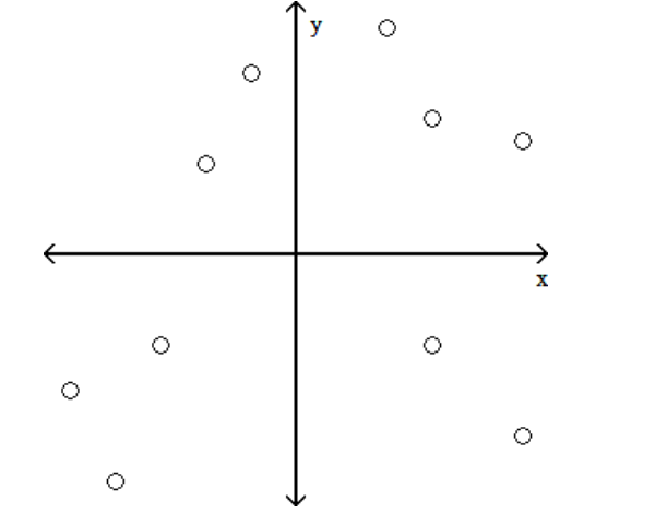
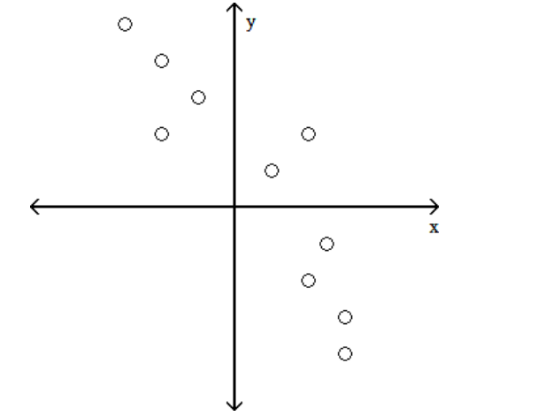
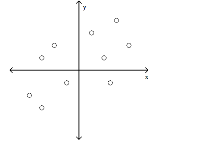
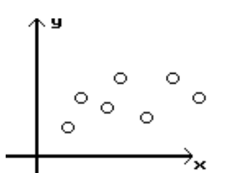
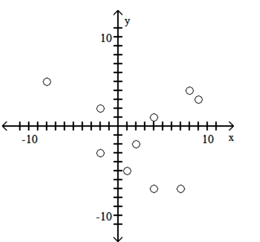
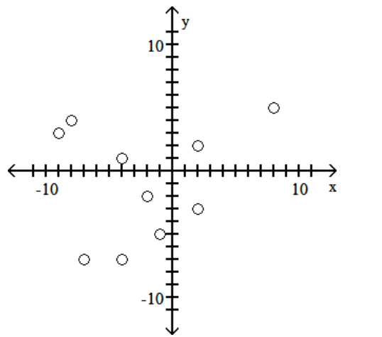
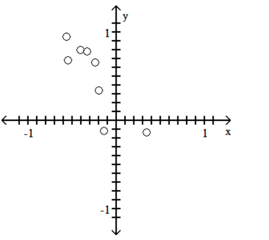
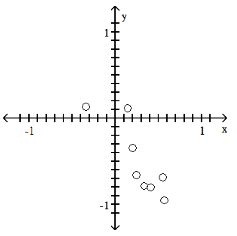
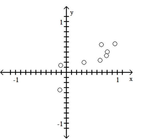
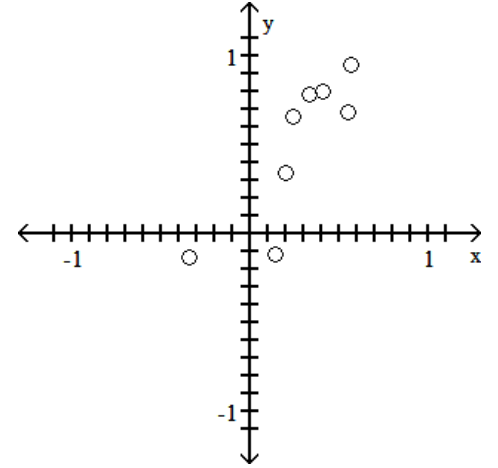
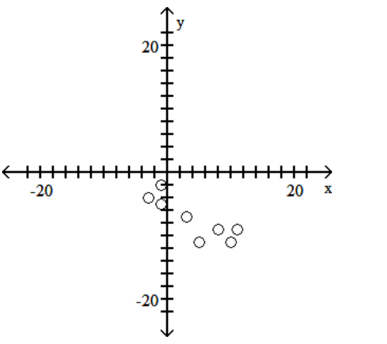
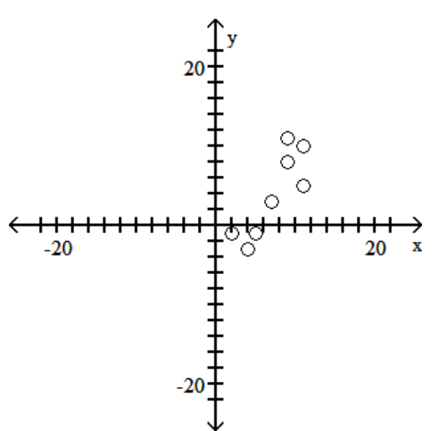
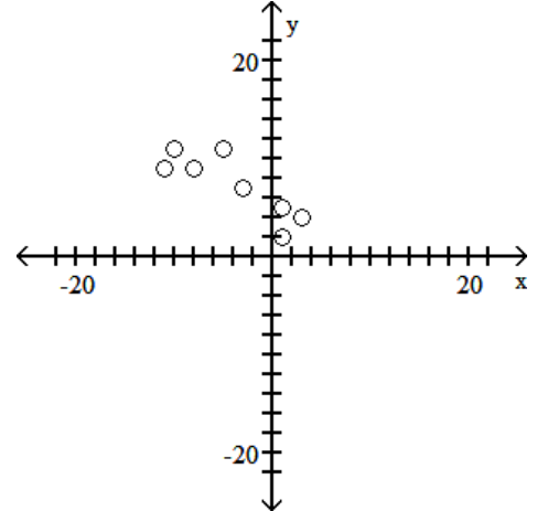
Determine which plot shows the strongest linear correlation.
A)
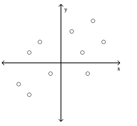
B)
C)
D)
A)
B)
C)
D)
Question
Question
Question
Question
Question
Question
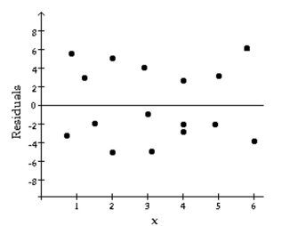
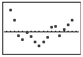
The following residual plot is obtained after a regression equation is determined for a set of data. Does the residual plot suggest that the regression equation is a bad model? Why or why not? 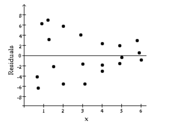
Question
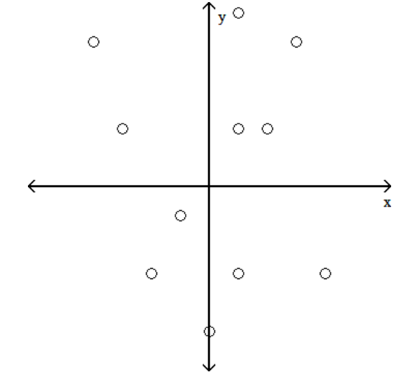
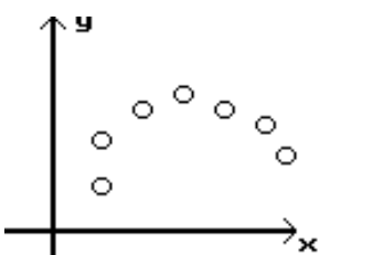
Which shows the strongest linear correlation?
A)
B)
C)
A)
B)
C)
Question
Question
Question
Question
Question
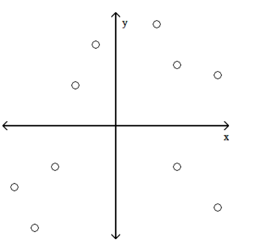
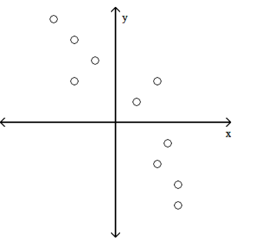
Determine which scatterplot shows the strongest linear correlation.
-Which shows the strongest linear correlation?
A)
B)
C)
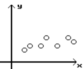
-Which shows the strongest linear correlation?
A)
B)
C)
Question
Question
Question
Question
Nine adults were selected at random from among those working full time in the town of Workington.
Each person was asked the number of years of college education they had completed and was also asked to rate their job satisfaction on a scale of 1 to 10.
The pairs of data values area plotted in the scatterplot below.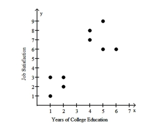
The four points in the lower left corner correspond to employees from company A and the five points in the upper right corner correspond to employees from company B.
a. Using the pairs of values for all 9 points, find the equation of the regression line.
b. Using only the pairs of values for the four points in the lower left corner, find the equation of the regression line.
c. Using only the pairs of values for the five points in the upper right corner, find the equation of the regression line.
d. Compare the results from parts a, b, and c.
Question
The sample data below are the typing speeds (in words per minute) and reading speeds (in words per minute) of nine randomly selected secretaries. Here, x denotes typing speed, and y denotes reading speed.
The regression equation was obtained. Construct a residual plot for the data.
The regression equation was obtained. Construct a residual plot for the data.
Question
Question
Question
Question
Question
Question
Question
Question
Question
Question
Question
Question
Question
Question
Question
Question
Question
Question
The following residual plot is obtained after a regression equation is determined for a set of data. Does the residual plot suggest that the regression equation is a bad model? Why or why not?
Question
Question
Question
Applicants for a particular job, which involves extensive travel in Spanish speaking countries, must take a proficiency test in Spanish. The sample data below were obtained in a study of the relationship between the numbers of years applicants have studied Spanish (x) and their score on the test (y).
Question
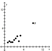
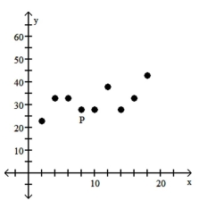
Is the data point, P, an outlier, an influential point, both, or neither?
A) Influential point
B) Neither
C) Outlier
D) Both
A) Influential point
B) Neither
C) Outlier
D) Both
Question
Question
The following table gives the US domestic oil production rates (excluding Alaska) over the past few years. A regression equation was fit to the data and the residual plot is shown below.
Does the residual plot suggest that the regression equation is a bad model? Why or why
not?
Does the residual plot suggest that the regression equation is a bad model? Why or why
not?
Question
Question
Question
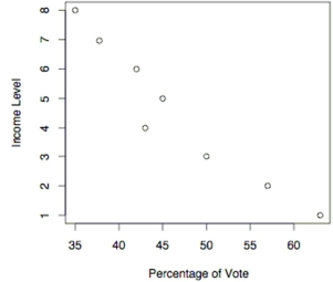
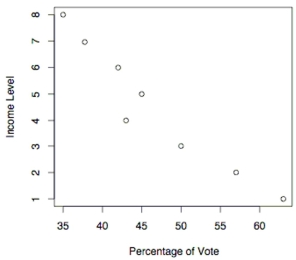
The following scatterplot shows the percentage of the vote a candidate received in the 2004 senatorial elections according to the voter's income level based on an exit poll of voters conducted by CNN. The income levels 1-8 correspond to the following income classes: Under ; or more.
-Use the election scatterplot to determine whether there is a correlation between percentage of vote and income level at the 0.01 significance level with a null hypothesis of
A) The test statistic is between the critical values, so we fail to reject the null hypothesis . There is no evidence to support a claim of correlation between percentage of vote and income level.
B) The test statistic is between the critical values, so we reject the null hypothesis . There is sufficient evidence to support a claim of correlation between percentage of vote and income level.
C) The test statistic is not between the critical values, so we fail to reject the null hypothesis . There is no evidence to support a claim of correlation between percentage of vote and income level.
D) The test statistic is not between the critical values, so we reject the null hypothesis . There is sufficient evidence to support a claim of correlation between percentage of vote and income level.
Question
Is the data point, P, an outlier, an influential point, both, or neither?
-
A) Influential point
B) Neither
C) Outlier
D) Both
-
A) Influential point
B) Neither
C) Outlier
D) Both
Question
The following scatterplot shows the percentage of the vote a candidate received in the 2004 senatorial elections according to the voter's income level based on an exit poll of voters conducted by CNN. The income levels 1-8 correspond to the following income classes: Under ; or more.
-Use the election scatterplot to the find the critical values corresponding to a significance level used to test the null hypothesis of .
A)
B) and
C)
D) and
-Use the election scatterplot to the find the critical values corresponding to a significance level used to test the null hypothesis of .
A)
B) and
C)
D) and
Question
Question
The following scatterplot shows the percentage of the vote a candidate received in the 2004 senatorial elections according to the voter's income level based on an exit poll of voters conducted by CNN. The income levels 1-8 correspond to the following income classes: Under ; or more.
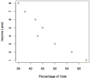
-Use the election scatterplot to the find the value of the rank correlation coefficient .
A)
B)
C)
D)
-Use the election scatterplot to the find the value of the rank correlation coefficient .
A)
B)
C)
D)
Question
Construct a scatterplot for the given data.
-
A)
B)
C)
D)
-
A)
B)
C)
D)
Question
Question
Question
Question
For which of the following sets of data points can you reasonably determine a regression line? 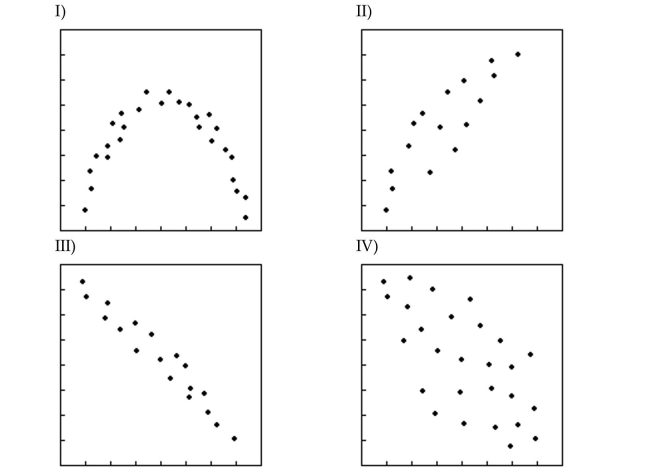
A) II, III, and IV
B) All of these
C) None of these
D) II and III
A) II, III, and IV
B) All of these
C) None of these
D) II and III
Question
Question
Question
Question
Question
Question
Question
Construct a scatterplot for the given data
-
A)
B)
C)
D)
-
A)
B)
C)
D)
Question
Question
Question
Question
Question
Question
Question
Question
Question
Question
Question
Question
A)
B)
C)
Question
Question
Question
Question
Question
Question

Unlock Deck
Sign up to unlock the cards in this deck!
Unlock Deck
Unlock Deck
1/104
Play
Full screen (f)
Deck 10: Correlation and Regression
1
For each of 200 randomly selected cities, Pete recorded the number of churches in the city (x) and the number of homicides in the past decade (y). He calculated the linear correlation coefficient and was surprised to find a strong positive linear correlation for the two variables. Does this suggest that building new churches causes an increase in the number of homicides? Why do you think that a strong positive linear correlation coefficient was
obtained? Explain your answer with reference to the term lurking variable.
obtained? Explain your answer with reference to the term lurking variable.
The positive linear correlation coefficient suggests that cities with a lot of churches also tend to have a high number of homicides. However, this does not imply causality. It does not imply that building new churches would cause an increase in the number of homicides. The correlation between the two variables is explained by their association with another variable (called a lurking variable), population. Larger cities tend to have both more churches and more homicides than small cities.
2
Determine which plot shows the strongest linear correlation.
A)
B)
C)
D)
A)
B)
C)
D)
3
A set of data consists of the number of years that applicants for foreign service jobs have studied German and the grades that they received on a proficiency test. The following regression equation is obtained: where x represents the number of years of study and y represents the grade on the test. Identify the predictor and response variables.
The predictor variable is the number of years of study, and the response variable is the grade on the test.
4
Define rank. Explain how to find the rank for data which repeats (for example, the data set:
4, 5, 5, 5, 7, 8, 12, 12, 15, 18).
4, 5, 5, 5, 7, 8, 12, 12, 15, 18).
Unlock Deck
Unlock for access to all 104 flashcards in this deck.
Unlock Deck
k this deck
5
A set of data consists of the number of years that applicants for foreign service jobs have studied German and the grades that they received on a proficiency test. The following regression equation is obtained: where x represents the number of years of study and y represents the grade on the test. What does the slope of the regression line represent in terms of grade on the test?
Unlock Deck
Unlock for access to all 104 flashcards in this deck.
Unlock Deck
k this deck
6
Describe the standard error of estimate, se. How do smaller values of se relate to the dispersion of data points about the line determined by the linear regression equation?
What does it mean when se is 0?
What does it mean when se is 0?
Unlock Deck
Unlock for access to all 104 flashcards in this deck.
Unlock Deck
k this deck
7
Given: There is no significant linear correlation between scores on a math test and scores on a verbal test.
Conclusion: There is no relationship between scores on the math test and scores on the verbal test.
Conclusion: There is no relationship between scores on the math test and scores on the verbal test.
Unlock Deck
Unlock for access to all 104 flashcards in this deck.
Unlock Deck
k this deck
8
The following residual plot is obtained after a regression equation is determined for a set of data. Does the residual plot suggest that the regression equation is a bad model? Why or why not?
Unlock Deck
Unlock for access to all 104 flashcards in this deck.
Unlock Deck
k this deck
9
Which shows the strongest linear correlation?
A)
B)
C)
A)
B)
C)
Unlock Deck
Unlock for access to all 104 flashcards in this deck.
Unlock Deck
k this deck
10
A regression equation is obtained for the following set of data. For what range of x-values
would it be reasonable to use the regression equation to predict the y-value? Why?
would it be reasonable to use the regression equation to predict the y-value? Why?
Unlock Deck
Unlock for access to all 104 flashcards in this deck.
Unlock Deck
k this deck
11
Describe the error in the stated conclusion
-Given: Each school in a state reports the average SAT score of its students. There is a significant linear correlation between the average SAT score of a school and the average annual income in the district in which the school is located.
Conclusion: There is a significant linear correlation between individual SAT scores and family income.
Unlock Deck
Unlock for access to all 104 flashcards in this deck.
Unlock Deck
k this deck
12
Use the rank correlation coefficient to test for a correlation between the two variables.
-A placement test is required for students desiring to take a finite mathematics course at a university. The instructor of the course studies the relationship between students' placement test score and final course score. A random sample of eight students yields the following data.
Compute the rank correlation coefficient, rs, of the data and test the claim of correlation between placement score and final course score. Use a significance level of 0.05.
Unlock Deck
Unlock for access to all 104 flashcards in this deck.
Unlock Deck
k this deck
13
Describe the rank correlation test. What types of hypotheses is it used to test? How does the rank correlation coefficient rs differ from the Pearson correlation coefficient r?
Unlock Deck
Unlock for access to all 104 flashcards in this deck.
Unlock Deck
k this deck
14
Determine which scatterplot shows the strongest linear correlation.
-Which shows the strongest linear correlation?
A)
B)
C)
-Which shows the strongest linear correlation?
A)
B)
C)
Unlock Deck
Unlock for access to all 104 flashcards in this deck.
Unlock Deck
k this deck
15
Explain what is meant by the coefficient of determination, . Give an example to support your result.
Unlock Deck
Unlock for access to all 104 flashcards in this deck.
Unlock Deck
k this deck
16
Given: There is a significant linear correlation between the number of homicides in a town and the number of movie theaters in a town.
Conclusion: Building more movie theaters will cause the homicide rate to rise.
Conclusion: Building more movie theaters will cause the homicide rate to rise.
Unlock Deck
Unlock for access to all 104 flashcards in this deck.
Unlock Deck
k this deck
17
Define the terms predictor variable and response variable. Give examples for each.
Unlock Deck
Unlock for access to all 104 flashcards in this deck.
Unlock Deck
k this deck
18
Nine adults were selected at random from among those working full time in the town of Workington.
Each person was asked the number of years of college education they had completed and was also asked to rate their job satisfaction on a scale of 1 to 10.
The pairs of data values area plotted in the scatterplot below.
The four points in the lower left corner correspond to employees from company A and the five points in the upper right corner correspond to employees from company B.
a. Using the pairs of values for all 9 points, find the equation of the regression line.
b. Using only the pairs of values for the four points in the lower left corner, find the equation of the regression line.
c. Using only the pairs of values for the five points in the upper right corner, find the equation of the regression line.
d. Compare the results from parts a, b, and c.
Each person was asked the number of years of college education they had completed and was also asked to rate their job satisfaction on a scale of 1 to 10.
The pairs of data values area plotted in the scatterplot below.
The four points in the lower left corner correspond to employees from company A and the five points in the upper right corner correspond to employees from company B.
a. Using the pairs of values for all 9 points, find the equation of the regression line.
b. Using only the pairs of values for the four points in the lower left corner, find the equation of the regression line.
c. Using only the pairs of values for the five points in the upper right corner, find the equation of the regression line.
d. Compare the results from parts a, b, and c.
Unlock Deck
Unlock for access to all 104 flashcards in this deck.
Unlock Deck
k this deck
19
The sample data below are the typing speeds (in words per minute) and reading speeds (in words per minute) of nine randomly selected secretaries. Here, x denotes typing speed, and y denotes reading speed.
The regression equation was obtained. Construct a residual plot for the data.
The regression equation was obtained. Construct a residual plot for the data.
Unlock Deck
Unlock for access to all 104 flashcards in this deck.
Unlock Deck
k this deck
20
For the data below, determine the value of the linear correlation coefficient r between y and ln x and test whether the linear correlation is significant. Use a significance level of0.05.
Unlock Deck
Unlock for access to all 104 flashcards in this deck.
Unlock Deck
k this deck
21
Ten trucks were ranked according to their comfort levels and their prices.
Find the rank correlation coefficient and test the claim of correlation between comfort and price. Use a significance level of 0.05.
Find the rank correlation coefficient and test the claim of correlation between comfort and price. Use a significance level of 0.05.
Unlock Deck
Unlock for access to all 104 flashcards in this deck.
Unlock Deck
k this deck
22
Suppose there is significant correlation between two variables. Describe two cases under which it might be inappropriate to use the linear regression equation for prediction. Give examples to support these cases.
Unlock Deck
Unlock for access to all 104 flashcards in this deck.
Unlock Deck
k this deck
23
Use the rank correlation coefficient to test for a correlation between the two variables.
-Use the sample data below to find the rank correlation coefficient and test the claim of correlation between math and verbal scores. Use a significance level of 0.05.
-Use the sample data below to find the rank correlation coefficient and test the claim of correlation between math and verbal scores. Use a significance level of 0.05.
Unlock Deck
Unlock for access to all 104 flashcards in this deck.
Unlock Deck
k this deck
24
Describe what scatterplots are and discuss the importance of creating scatterplots.
Unlock Deck
Unlock for access to all 104 flashcards in this deck.
Unlock Deck
k this deck
25
Use the rank correlation coefficient to test for a correlation between the two variables.
-Given that the rank correlation coefficient, rs, for 73 pairs of data is -0.663, test the claim of correlation between the two variables. Use a significance level of 0.05.
-Given that the rank correlation coefficient, rs, for 73 pairs of data is -0.663, test the claim of correlation between the two variables. Use a significance level of 0.05.
Unlock Deck
Unlock for access to all 104 flashcards in this deck.
Unlock Deck
k this deck
26
Explain why having a significant linear correlation does not imply causality. Give an example to support your answer.
Unlock Deck
Unlock for access to all 104 flashcards in this deck.
Unlock Deck
k this deck
27
Use the rank correlation coefficient to test for a correlation between the two variables.
-The scores of twelve students on the midterm exam and the final exam were as follows.
Find the rank correlation coefficient and test the claim of correlation between midterm score and final exam score. Use a significance level of 0.05.
-The scores of twelve students on the midterm exam and the final exam were as follows.
Find the rank correlation coefficient and test the claim of correlation between midterm score and final exam score. Use a significance level of 0.05.
Unlock Deck
Unlock for access to all 104 flashcards in this deck.
Unlock Deck
k this deck
28
The variables height and weight could reasonably be expected to have a positive linear correlation coefficient, since taller people tend to be heavier, on average, than shorter people. Give an example of a pair of variables which you would expect to have a negative linear correlation coefficient and explain why. Then give an example of a pair of variables whose linear correlation coefficient is likely to be close to zero.
Unlock Deck
Unlock for access to all 104 flashcards in this deck.
Unlock Deck
k this deck
29
Use the rank correlation coefficient to test for a correlation between the two variables.
-A college administrator collected information on first-semester night-school students. A random sample taken of 12 students yielded the following data on age and GPA during the first semester.
Do the data provide sufficient evidence to conclude that the variables age, , and GPA, , are correlated? Apply a rank-correlation test. Use .
Unlock Deck
Unlock for access to all 104 flashcards in this deck.
Unlock Deck
k this deck
30
A regression equation is obtained for a set of data. After examining a scatter diagram, the researcher notices a data point that is potentially an influential point. How could she confirm that this data point is indeed an influential point?
Unlock Deck
Unlock for access to all 104 flashcards in this deck.
Unlock Deck
k this deck
31
Suppose paired data are collected consisting of, for each person, their weight in pounds and the number of calories burned in 30 minutes of walking on a treadmill at 3.5 mph.
How would the value of the correlation coefficient, r, change if all of the weights were converted to kilograms?
How would the value of the correlation coefficient, r, change if all of the weights were converted to kilograms?
Unlock Deck
Unlock for access to all 104 flashcards in this deck.
Unlock Deck
k this deck
32
Use the rank correlation coefficient to test for a correlation between the two variables.
-Ten luxury cars were ranked according to their comfort levels and their prices.
Find the rank correlation coefficient and test the claim of correlation between comfort and price. Use a significance level of 0.05.
-Ten luxury cars were ranked according to their comfort levels and their prices.
Find the rank correlation coefficient and test the claim of correlation between comfort and price. Use a significance level of 0.05.
Unlock Deck
Unlock for access to all 104 flashcards in this deck.
Unlock Deck
k this deck
33
Given: The linear correlation coefficient between scores on a math test and scores on a test of athletic ability is negative and close to zero.
Conclusion: People who score high on the math test tend to score lower on the test of athletic ability.
Conclusion: People who score high on the math test tend to score lower on the test of athletic ability.
Unlock Deck
Unlock for access to all 104 flashcards in this deck.
Unlock Deck
k this deck
34
Create a scatterplot that shows a perfect positive correlation between x and y. How would the scatterplot change if the correlation showed a) a strong positive correlation, b) a weak positive correlation, and c) no correlation?
Unlock Deck
Unlock for access to all 104 flashcards in this deck.
Unlock Deck
k this deck
35
Given that the rank correlation coefficien for 15 pairs of data is -0.636, test the claim of correlation between the two variables. Use a significance level of 0.01.
Unlock Deck
Unlock for access to all 104 flashcards in this deck.
Unlock Deck
k this deck
36
Use the rank correlation coefficient to test for a correlation between the two variables.
-Given that the rank correlation coefficient, r , for 33 pairs of data is 0.338, test the claim of
correlation between the two variables. Use a significance level of 0.01.
-Given that the rank correlation coefficient, r , for 33 pairs of data is 0.338, test the claim of
correlation between the two variables. Use a significance level of 0.01.
Unlock Deck
Unlock for access to all 104 flashcards in this deck.
Unlock Deck
k this deck
37
The following residual plot is obtained after a regression equation is determined for a set of data. Does the residual plot suggest that the regression equation is a bad model? Why or why not?
Unlock Deck
Unlock for access to all 104 flashcards in this deck.
Unlock Deck
k this deck
38
What is the relationship between the linear correlation coefficient and the usefulness of the regression equation for making predictions?
Unlock Deck
Unlock for access to all 104 flashcards in this deck.
Unlock Deck
k this deck
39
Discuss the guidelines under which the linear regression equation should be used for prediction. Refer to the correlation coefficient and the value of the predictor variable.
Unlock Deck
Unlock for access to all 104 flashcards in this deck.
Unlock Deck
k this deck
40
Applicants for a particular job, which involves extensive travel in Spanish speaking countries, must take a proficiency test in Spanish. The sample data below were obtained in a study of the relationship between the numbers of years applicants have studied Spanish (x) and their score on the test (y).
Unlock Deck
Unlock for access to all 104 flashcards in this deck.
Unlock Deck
k this deck
41
Is the data point, P, an outlier, an influential point, both, or neither?
A) Influential point
B) Neither
C) Outlier
D) Both
A) Influential point
B) Neither
C) Outlier
D) Both
Unlock Deck
Unlock for access to all 104 flashcards in this deck.
Unlock Deck
k this deck
42
Is the data point, P, an outlier, an influential point, both, or neither?
-The regression equation for a set of paired data is . The values of x run from 100 to 400. A new data point, P(176, 159.1), is added to the set.
A) Neither
B) Both
C) Outlier
D) Influential point
-The regression equation for a set of paired data is . The values of x run from 100 to 400. A new data point, P(176, 159.1), is added to the set.
A) Neither
B) Both
C) Outlier
D) Influential point
Unlock Deck
Unlock for access to all 104 flashcards in this deck.
Unlock Deck
k this deck
43
The following table gives the US domestic oil production rates (excluding Alaska) over the past few years. A regression equation was fit to the data and the residual plot is shown below.
Does the residual plot suggest that the regression equation is a bad model? Why or why
not?
Does the residual plot suggest that the regression equation is a bad model? Why or why
not?
Unlock Deck
Unlock for access to all 104 flashcards in this deck.
Unlock Deck
k this deck
44
When performing a rank correlation test, one alternative to using the Critical Values of Spearman's Rank Correlation Coefficient table to find critical values is to compute them using this approximation
where is the -score from the Distribution table corresponding to degrees of freedom. Use this approximation to find critical values of for the case where and .
A)
B)
C)
D)
where is the -score from the Distribution table corresponding to degrees of freedom. Use this approximation to find critical values of for the case where and .
A)
B)
C)
D)
Unlock Deck
Unlock for access to all 104 flashcards in this deck.
Unlock Deck
k this deck
45
Use the rank correlation coefficient to test for a correlation between the two variables.
-Given that the rank correlation coefficient, r for 20 pairs of data is 0.827, test the claim of correlation between the two variables. Use a significance level of 0.05.
-Given that the rank correlation coefficient, r for 20 pairs of data is 0.827, test the claim of correlation between the two variables. Use a significance level of 0.05.
Unlock Deck
Unlock for access to all 104 flashcards in this deck.
Unlock Deck
k this deck
46
The following scatterplot shows the percentage of the vote a candidate received in the 2004 senatorial elections according to the voter's income level based on an exit poll of voters conducted by CNN. The income levels 1-8 correspond to the following income classes: Under ; or more.
-Use the election scatterplot to determine whether there is a correlation between percentage of vote and income level at the 0.01 significance level with a null hypothesis of
A) The test statistic is between the critical values, so we fail to reject the null hypothesis . There is no evidence to support a claim of correlation between percentage of vote and income level.
B) The test statistic is between the critical values, so we reject the null hypothesis . There is sufficient evidence to support a claim of correlation between percentage of vote and income level.
C) The test statistic is not between the critical values, so we fail to reject the null hypothesis . There is no evidence to support a claim of correlation between percentage of vote and income level.
D) The test statistic is not between the critical values, so we reject the null hypothesis . There is sufficient evidence to support a claim of correlation between percentage of vote and income level.
Unlock Deck
Unlock for access to all 104 flashcards in this deck.
Unlock Deck
k this deck
47
Is the data point, P, an outlier, an influential point, both, or neither?
-
A) Influential point
B) Neither
C) Outlier
D) Both
-
A) Influential point
B) Neither
C) Outlier
D) Both
Unlock Deck
Unlock for access to all 104 flashcards in this deck.
Unlock Deck
k this deck
48
The following scatterplot shows the percentage of the vote a candidate received in the 2004 senatorial elections according to the voter's income level based on an exit poll of voters conducted by CNN. The income levels 1-8 correspond to the following income classes: Under ; or more.
-Use the election scatterplot to the find the critical values corresponding to a significance level used to test the null hypothesis of .
A)
B) and
C)
D) and
-Use the election scatterplot to the find the critical values corresponding to a significance level used to test the null hypothesis of .
A)
B) and
C)
D) and
Unlock Deck
Unlock for access to all 104 flashcards in this deck.
Unlock Deck
k this deck
49
Two different tests are designed to measure employee productivity and dexterity. Several employees are randomly selected and tested with these results.
A) 0.115
B) 0.986
C) 0.471
D) - 0.280
A) 0.115
B) 0.986
C) 0.471
D) - 0.280
Unlock Deck
Unlock for access to all 104 flashcards in this deck.
Unlock Deck
k this deck
50
The following scatterplot shows the percentage of the vote a candidate received in the 2004 senatorial elections according to the voter's income level based on an exit poll of voters conducted by CNN. The income levels 1-8 correspond to the following income classes: Under ; or more.
-Use the election scatterplot to the find the value of the rank correlation coefficient .
A)
B)
C)
D)
-Use the election scatterplot to the find the value of the rank correlation coefficient .
A)
B)
C)
D)
Unlock Deck
Unlock for access to all 104 flashcards in this deck.
Unlock Deck
k this deck
51
Construct a scatterplot for the given data.
-
A)
B)
C)
D)
-
A)
B)
C)
D)
Unlock Deck
Unlock for access to all 104 flashcards in this deck.
Unlock Deck
k this deck
52
For the data below, determine the value of the linear correlation coefficient between and .
A)
B)
C)
D)
A)
B)
C)
D)
Unlock Deck
Unlock for access to all 104 flashcards in this deck.
Unlock Deck
k this deck
53
Find the value of the linear correlation coefficient r.
-
A) 0.214
B) -0.078
C) -0.054
D) 0.109
-
A) 0.214
B) -0.078
C) -0.054
D) 0.109
Unlock Deck
Unlock for access to all 104 flashcards in this deck.
Unlock Deck
k this deck
54
Given the linear correlation coefficient r and the sample size n, determine the critical values of r and use your finding to state whether or not the given r represents a significant linear correlation. Use a significance level of 0.05.
-
A) Critical values: , no significant linear correlation
B) Critical values: , no significant linear correlation
C) Critical values: , significant linear correlation
D) Critical values: , no significant linear correlation
-
A) Critical values: , no significant linear correlation
B) Critical values: , no significant linear correlation
C) Critical values: , significant linear correlation
D) Critical values: , no significant linear correlation
Unlock Deck
Unlock for access to all 104 flashcards in this deck.
Unlock Deck
k this deck
55
For which of the following sets of data points can you reasonably determine a regression line?
A) II, III, and IV
B) All of these
C) None of these
D) II and III
A) II, III, and IV
B) All of these
C) None of these
D) II and III
Unlock Deck
Unlock for access to all 104 flashcards in this deck.
Unlock Deck
k this deck
56
When performing a rank correlation test, one alternative to using the Critical Values of Spearman's Rank Correlation Coefficient table to find critical values is to compute them using this approximation:
where is the -score from the Distribution table corresponding to degrees of freedom. Use this approximation to find critical values of for the case where and .
A)
B)
C)
D)
where is the -score from the Distribution table corresponding to degrees of freedom. Use this approximation to find critical values of for the case where and .
A)
B)
C)
D)
Unlock Deck
Unlock for access to all 104 flashcards in this deck.
Unlock Deck
k this deck
57
Find the value of the linear correlation coefficient r.
-Two separate tests are designed to measure a student's ability to solve problems. Several students are randomly selected to take both tests and the results are shown below.
A) 0.109
B) 0.714
C) 0.548
D) 0.867
-Two separate tests are designed to measure a student's ability to solve problems. Several students are randomly selected to take both tests and the results are shown below.
A) 0.109
B) 0.714
C) 0.548
D) 0.867
Unlock Deck
Unlock for access to all 104 flashcards in this deck.
Unlock Deck
k this deck
58
Use the given data to find the best predicted value of the response variable.
-Eight pairs of data yield and the regression equation . Also, What is the best predicted value of for
A) 71.13
B) 83.42
C) 555.21
D) 57.80
-Eight pairs of data yield and the regression equation . Also, What is the best predicted value of for
A) 71.13
B) 83.42
C) 555.21
D) 57.80
Unlock Deck
Unlock for access to all 104 flashcards in this deck.
Unlock Deck
k this deck
59
The paired data below consist of the test scores of 6 randomly selected students and the number of hours they studied for the test.
A) 0.224
B) -0.224
C) -0.678
D) 0.678
A) 0.224
B) -0.224
C) -0.678
D) 0.678
Unlock Deck
Unlock for access to all 104 flashcards in this deck.
Unlock Deck
k this deck
60
The regression equation for a set of paired data is . The correlation coefficient for the data is 0.87. A new data point, P(12, 53), is added to the set.
A) Outlier
B) Influential point
C) Both
D) Neither
A) Outlier
B) Influential point
C) Both
D) Neither
Unlock Deck
Unlock for access to all 104 flashcards in this deck.
Unlock Deck
k this deck
61
Given the linear correlation coefficient r and the sample size n, determine the critical values of r and use your finding to state whether or not the given r represents a significant linear correlation. Use a significance level of 0.05.
-
A) Critical values: , significant linear correlation
B) Critical values: , no significant linear correlation
C) Critical values: , no significant linear correlation
D) Critical values: , no significant linear correlation
-
A) Critical values: , significant linear correlation
B) Critical values: , no significant linear correlation
C) Critical values: , no significant linear correlation
D) Critical values: , no significant linear correlation
Unlock Deck
Unlock for access to all 104 flashcards in this deck.
Unlock Deck
k this deck
62
Construct a scatterplot for the given data
-
A)
B)
C)
D)
-
A)
B)
C)
D)
Unlock Deck
Unlock for access to all 104 flashcards in this deck.
Unlock Deck
k this deck
63
Find the value of the linear correlation coefficient r.
-The paired data below consist of the temperatures on randomly chosen days and the amount a certain kind of plant grew (in millimeters):
A) -0.210
B) 0.256
C) 0.196
D) 0
-The paired data below consist of the temperatures on randomly chosen days and the amount a certain kind of plant grew (in millimeters):
A) -0.210
B) 0.256
C) 0.196
D) 0
Unlock Deck
Unlock for access to all 104 flashcards in this deck.
Unlock Deck
k this deck
64
A study was conducted to compare the average time spent in the lab each week versus course grade for computer programming students. The results are recorded in the table below.
A)
B)
C)
D)
A)
B)
C)
D)
Unlock Deck
Unlock for access to all 104 flashcards in this deck.
Unlock Deck
k this deck
65
Find the critical value. Assume that the test is two-tailed and that n denotes the number of pairs of data.
-
A)
B)
C)
D)
-
A)
B)
C)
D)
Unlock Deck
Unlock for access to all 104 flashcards in this deck.
Unlock Deck
k this deck
66
When performing a rank correlation test, one alternative to using the Critical Values of Spearman's Rank Correlation Coefficient table to find critical values is to compute them using this approximation:
where is the -score from the Distribution table corresponding to degrees of freedom. Use this approximation to find critical values of for the case where and .
A)
B)
C)
D)
where is the -score from the Distribution table corresponding to degrees of freedom. Use this approximation to find critical values of for the case where and .
A)
B)
C)
D)
Unlock Deck
Unlock for access to all 104 flashcards in this deck.
Unlock Deck
k this deck
67
Find the critical value. Assume that the test is two-tailed and that n denotes the number of pairs of data.
-
A)
B)
C)
D)
-
A)
B)
C)
D)
Unlock Deck
Unlock for access to all 104 flashcards in this deck.
Unlock Deck
k this deck
68
Use the given data to find the equation of the regression line. Round the final values to three significant digits, if necessary.
-
A)
B)
C)
D)
-
A)
B)
C)
D)
Unlock Deck
Unlock for access to all 104 flashcards in this deck.
Unlock Deck
k this deck
69
Use the given data to find the best predicted value of the response variable.
-Four pairs of data yield and the regression equation . Also, . What is the best predicted value of for ?
A) 0.942
B) 2.826
C) 12.75
D) 17.4
-Four pairs of data yield and the regression equation . Also, . What is the best predicted value of for ?
A) 0.942
B) 2.826
C) 12.75
D) 17.4
Unlock Deck
Unlock for access to all 104 flashcards in this deck.
Unlock Deck
k this deck
70
Which of the following statements concerning the linear correlation coefficient are true? I: If the linear correlation coefficient for two variables is zero, then there is no relationship between The variables.
II: If the slope of the regression line is negative, then the linear correlation coefficient is negative.
III: The value of the linear correlation coefficient always lies between -1 and 1.
IV: A linear correlation coefficient of 0.62 suggests a stronger linear relationship than a linear Correlation coefficient of -0.82.
A) III and IV
B) I and II
C) II and III
D) I and IV
Unlock Deck
Unlock for access to all 104 flashcards in this deck.
Unlock Deck
k this deck
71
Use the given data to find the equation of the regression line. Round the final values to three significant digits, if necessary.
-
A)
B)
C)
D)
-
A)
B)
C)
D)
Unlock Deck
Unlock for access to all 104 flashcards in this deck.
Unlock Deck
k this deck
72
Use the given data to find the equation of the regression line. Round the final values to three significant digits, if necessary.
-
A)
B)
C)
D)
-
A)
B)
C)
D)
Unlock Deck
Unlock for access to all 104 flashcards in this deck.
Unlock Deck
k this deck
73
Given the linear correlation coefficient r and the sample size n, determine the critical values of r and use your finding to state whether or not the given r represents a significant linear correlation. Use a significance level of 0.05.
-
A) Critical values: , no significant linear correlation
B) Critical values: , no significant linear correlation
C) Critical values: , significant linear correlation
D) Critical values: , significant linear correlation
-
A) Critical values: , no significant linear correlation
B) Critical values: , no significant linear correlation
C) Critical values: , significant linear correlation
D) Critical values: , significant linear correlation
Unlock Deck
Unlock for access to all 104 flashcards in this deck.
Unlock Deck
k this deck
74
A)
B)
C)
Unlock Deck
Unlock for access to all 104 flashcards in this deck.
Unlock Deck
k this deck
75
Ten students in a graduate program were randomly selected. Their grade point averages (GPAs) when they entered the program were between 3.5 and 4.0. The following data were obtained regarding their GPAs on entering the program versus their current GPAs.
A)
B)
C)
D)
A)
B)
C)
D)
Unlock Deck
Unlock for access to all 104 flashcards in this deck.
Unlock Deck
k this deck
76
Use the given data to find the best predicted value of the response variable.
-Six pairs of data yield and the regression equation . Also, . What is the best predicted value of for ?
A) 93.5
B) 4.22
C) 18.3
D) 27
-Six pairs of data yield and the regression equation . Also, . What is the best predicted value of for ?
A) 93.5
B) 4.22
C) 18.3
D) 27
Unlock Deck
Unlock for access to all 104 flashcards in this deck.
Unlock Deck
k this deck
77
Find the value of the linear correlation coefficient r.
-Managers rate employees according to job performance and attitude. The results for several randomly selected employees are given below.
A) 0.610
B) 0.863
C) 0.729
D) 0.916
-Managers rate employees according to job performance and attitude. The results for several randomly selected employees are given below.
A) 0.610
B) 0.863
C) 0.729
D) 0.916
Unlock Deck
Unlock for access to all 104 flashcards in this deck.
Unlock Deck
k this deck
78
Use the given data to find the equation of the regression line. Round the final values to three significant digits, if necessary.
-Managers rate employees according to job performance and attitude. The results for several randomly selected employees are given below.
A)
B)
C)
D)
-Managers rate employees according to job performance and attitude. The results for several randomly selected employees are given below.
A)
B)
C)
D)
Unlock Deck
Unlock for access to all 104 flashcards in this deck.
Unlock Deck
k this deck
79
Find the critical value. Assume that the test is two-tailed and that n denotes the number of pairs of data.
-
A)
B)
C)
D)
-
A)
B)
C)
D)
Unlock Deck
Unlock for access to all 104 flashcards in this deck.
Unlock Deck
k this deck
80
Suppose you will perform a test to determine whether there is sufficient evidence to support a claim of a linear correlation between two variables. Find the critical values of r given the number of pairs of data n and the significance
level
-
A)
B)
C)
D)
level
-
A)
B)
C)
D)
Unlock Deck
Unlock for access to all 104 flashcards in this deck.
Unlock Deck
k this deck
Unlock Deck
Unlock for access to all 104 flashcards in this deck.


