Deck 4: Regression
Full screen (f)
Question
Question
Question
Question
Question
Tail-feather length in birds is sometimes a sexually dimorphic trait. That is, the trait differs substantially for males and for females. Researchers studied the relationship between tail-feather length (measuring the R1 central tail feather) and weight in a sample of 20 male and 21 female long-tailed finches raised in an aviary.
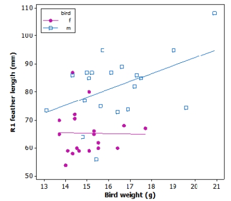 What is the value of the y intercept for the male regression line (blue squares)?
A)Approximately 70 mm
B)Less than 50 mm
C)0 mm
D)Cannot be guessed from the graph
What is the value of the y intercept for the male regression line (blue squares)?A)Approximately 70 mm
B)Less than 50 mm
C)0 mm
D)Cannot be guessed from the graph
Question
Tail-feather length in birds is sometimes a sexually dimorphic trait. That is, the trait differs substantially for males and for females. Researchers studied the relationship between tail-feather length (measuring the R1 central tail feather) and weight in a sample of 20 male and 21 female long-tailed finches raised in an aviary.
 What is the approximate value of the slope for the male regression line (blue squares)?
A)3 g/mm
B)3 mm/g
C)0.35 mm/g
D)0.35 g/mm
What is the approximate value of the slope for the male regression line (blue squares)?A)3 g/mm
B)3 mm/g
C)0.35 mm/g
D)0.35 g/mm
Question
Tail-feather length in birds is sometimes a sexually dimorphic trait. That is, the trait differs substantially for males and for females. Researchers studied the relationship between tail-feather length (measuring the R1 central tail feather) and weight in a sample of 20 male and 21 female long-tailed finches raised in an aviary.
 Which of the following statements is NOT true?
A)Male birds that are heavier tend to have longer tail feathers.
B)The ranges of weight typical of male and female birds are similar.
C)Overall, females tend to have smaller tail feathers than males, for a given body weight.
D)Both males and females show a clear positive linear relationship between weight and tail-feather length.
Which of the following statements is NOT true?A)Male birds that are heavier tend to have longer tail feathers.
B)The ranges of weight typical of male and female birds are similar.
C)Overall, females tend to have smaller tail feathers than males, for a given body weight.
D)Both males and females show a clear positive linear relationship between weight and tail-feather length.
Question
Tail-feather length in birds is sometimes a sexually dimorphic trait. That is, the trait differs substantially for males and for females. Researchers studied the relationship between tail-feather length (measuring the R1 central tail feather) and weight in a sample of 20 male and 21 female long-tailed finches raised in an aviary.
 What is a practical interpretation of the slope estimate of the least squares regression line for males (blue squares)?
A)For each additional gram of weight, we estimate the tail feather length to increase by 3 mm, on average.
B)For each additional gram of weight, we estimate the tail feather length to increase by 70 mm, on average.
C)For each additional millimeter of length of tail feather, we estimate weight to increase by 3 g, on average.
D)For each additional millimeter of length of tail feather, we estimate weight to increase by 70 g, on average.
What is a practical interpretation of the slope estimate of the least squares regression line for males (blue squares)?A)For each additional gram of weight, we estimate the tail feather length to increase by 3 mm, on average.
B)For each additional gram of weight, we estimate the tail feather length to increase by 70 mm, on average.
C)For each additional millimeter of length of tail feather, we estimate weight to increase by 3 g, on average.
D)For each additional millimeter of length of tail feather, we estimate weight to increase by 70 g, on average.
Question
Tail-feather length in birds is sometimes a sexually dimorphic trait. That is, the trait differs substantially for males and for females. Researchers studied the relationship between tail-feather length (measuring the R1 central tail feather) and weight in a sample of 20 male and 21 female long-tailed finches raised in an aviary.
 What is a meaningful interpretation in context of the estimate of the y intercept of the least squares line for males (blue squares)?
A)There is no meaningful interpretation, since a bird with 0 weight is not possible.
B)For each additional gram of weight, we estimate the tail feather length to increase by 3 mm, on average.
C)For each additional gram of weight, we estimate the tail feather length to increase by 70 mm, on average.
D)We estimate the tail feather length to be 70 mm, on average.
What is a meaningful interpretation in context of the estimate of the y intercept of the least squares line for males (blue squares)?A)There is no meaningful interpretation, since a bird with 0 weight is not possible.
B)For each additional gram of weight, we estimate the tail feather length to increase by 3 mm, on average.
C)For each additional gram of weight, we estimate the tail feather length to increase by 70 mm, on average.
D)We estimate the tail feather length to be 70 mm, on average.
Question
Tail-feather length in birds is sometimes a sexually dimorphic trait. That is, the trait differs substantially for males and for females. Researchers studied the relationship between tail-feather length (measuring the R1 central tail feather) and weight in a sample of 20 male and 21 female long-tailed finches raised in an aviary.
 The linear correlation coefficient (r) between weight and tail-feather length in male long-tailed finches is 0.46. Approximately what percent of variation in tail-feather length can be explained by weight among male long-tailed finches?
A)21%
B)46%
C)68%
D)92%
The linear correlation coefficient (r) between weight and tail-feather length in male long-tailed finches is 0.46. Approximately what percent of variation in tail-feather length can be explained by weight among male long-tailed finches?A)21%
B)46%
C)68%
D)92%
Question
Tail-feather length in birds is sometimes a sexually dimorphic trait. That is, the trait differs substantially for males and for females. Researchers studied the relationship between tail-feather length (measuring the R1 central tail feather) and weight in a sample of 20 male and 21 female long-tailed finches raised in an aviary.
 We would like to use the observed least-squares regression line between weight and tail-feather length of males to predict the tail-feather length of a male long-tailed finch weighing 28 g. Would this use be appropriate?
A)Yes, because the corresponding relationship is clearly linear
B)No, because the observed relationship is different for males and for females
C)No, because it would be extrapolating beyond range
D)No, because there is too much variation in the observed relationship
We would like to use the observed least-squares regression line between weight and tail-feather length of males to predict the tail-feather length of a male long-tailed finch weighing 28 g. Would this use be appropriate?A)Yes, because the corresponding relationship is clearly linear
B)No, because the observed relationship is different for males and for females
C)No, because it would be extrapolating beyond range
D)No, because there is too much variation in the observed relationship
Question
Tail-feather length in birds is sometimes a sexually dimorphic trait. That is, the trait differs substantially for males and for females. Researchers studied the relationship between tail-feather length (measuring the R1 central tail feather) and weight in a sample of 20 male and 21 female long-tailed finches raised in an aviary.
 We would like to use the observed least-squares regression line between weight and tail-feather length of females to predict the tail-feather length of a male long-tailed finch weighing 8 g. Would this prediction be appropriate?
A)Yes, because the corresponding relationship is clearly linear
B)No, because the observed relationship is different for males and for females
C)No, because it would be extrapolating beyond range
D)No, because there is too much variation in the observed relationship
We would like to use the observed least-squares regression line between weight and tail-feather length of females to predict the tail-feather length of a male long-tailed finch weighing 8 g. Would this prediction be appropriate?A)Yes, because the corresponding relationship is clearly linear
B)No, because the observed relationship is different for males and for females
C)No, because it would be extrapolating beyond range
D)No, because there is too much variation in the observed relationship
Question
Question
Question
Question
Question
Question
Question
Question
Question
Question
Question
Question
Question
Question
In a study of diet, the amount of weight lost and the starting weight for each individual was recorded. A scatterplot of the data is provided. The correlation between weight lost and starting weight was computed to be 0.934.
 What can be conclude about these data?
A)Weight lost can be accurately predicted from starting weight.
B)Starting weight can be accurately predicted from weight lost.
C)There is a very influential observation in the data.
D)All of these answers are correct.
What can be conclude about these data?A)Weight lost can be accurately predicted from starting weight.
B)Starting weight can be accurately predicted from weight lost.
C)There is a very influential observation in the data.
D)All of these answers are correct.
Question
In a study of diet, the amount of weight lost and the starting weight for each individual was recorded. A scatterplot of the data is provided. The correlation between weight lost and starting weight was computed to be 0.934.
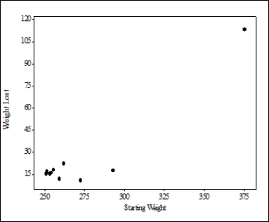 Because the correlation between starting weight and weight lost is so high, what can we conclude?
A)Having a high starting weight will cause a person to lose a lot of weight.
B)The slope of the least-squares regression line will be much larger than 1.
C)There is a strong, positive linear association between starting weight and weight lost, but this association may be largely driven by an influential observation.
D)Approximately 93% of the variability in weight lost is due to a person's starting weight.
Because the correlation between starting weight and weight lost is so high, what can we conclude?A)Having a high starting weight will cause a person to lose a lot of weight.
B)The slope of the least-squares regression line will be much larger than 1.
C)There is a strong, positive linear association between starting weight and weight lost, but this association may be largely driven by an influential observation.
D)Approximately 93% of the variability in weight lost is due to a person's starting weight.
Question
Question
Question
Question
Question
Tail-feather length in birds is sometimes a sexually dimorphic trait. That is, the trait differs substantially for males and for females. Researchers studied the relationship between tail-feather length (measuring the R1 central tail feather) and weight in a sample of 20 male long-tailed finches raised in an aviary. The data are represented in the following scatterplot, along with the least-squares regression line equation and the square of the correlation coefficient (R2).
 What is the value of the slope for the male regression line?
A)2.8299 g/mm
B)2.8299 mm/g
C)35.738 mm/g
D)35.738 g/mm
What is the value of the slope for the male regression line?A)2.8299 g/mm
B)2.8299 mm/g
C)35.738 mm/g
D)35.738 g/mm
Question
Tail-feather length in birds is sometimes a sexually dimorphic trait. That is, the trait differs substantially for males and for females. Researchers studied the relationship between tail-feather length (measuring the R1 central tail feather) and weight in a sample of 20 male long-tailed finches raised in an aviary. The data are represented in the following scatterplot, along with the least-squares regression line equation and the square of the correlation coefficient (R2).
 What is the value of the correlation coefficient describing the relationship between weight and tail-feather length?
A)Approximately 0.05
B)Approximately 0.21
C)Approximately 0.46
D)Cannot be estimated from the information provided
What is the value of the correlation coefficient describing the relationship between weight and tail-feather length?A)Approximately 0.05
B)Approximately 0.21
C)Approximately 0.46
D)Cannot be estimated from the information provided
Question
Tail-feather length in birds is sometimes a sexually dimorphic trait. That is, the trait differs substantially for males and for females. Researchers studied the relationship between tail-feather length (measuring the R1 central tail feather) and weight in a sample of 20 male long-tailed finches raised in an aviary. The data are represented in the following scatterplot, along with the least-squares regression line equation and the square of the correlation coefficient (R2).
 What would be the predicted tail-feather length of a male long-tailed finch weighing 20 g?
A)56.6 mm
B)92.3 mm
C)717.6 mm
D)Cannot be determined from the information given
What would be the predicted tail-feather length of a male long-tailed finch weighing 20 g?A)56.6 mm
B)92.3 mm
C)717.6 mm
D)Cannot be determined from the information given
Question
Question
Question
Question
Question
Question
Question

Unlock Deck
Sign up to unlock the cards in this deck!
Unlock Deck
Unlock Deck
1/41
Play
Full screen (f)
Deck 4: Regression
1
Before surgical removal of a diseased parathyroid gland, two tests are often performed: the standard intact test and the turbo test. Both tests measure parathyroid hormone (PTH, in ng/l), but the turbo test is very expensive. Researchers obtained data from both tests in a sample of 48 patients to predict turbo test results (y) from standard intact test results (x). The data ranged from roughly 0 to 500 ng/l, and a scatterplot showed a clear linear relationship. The published findings are summarized exactly as follows:
Y = 1.08x - 4.36 (r = 0.97; n = 48)
What is the slope of the regression line?
A)-4.36
B)0.97
C)1.08
D)48
Y = 1.08x - 4.36 (r = 0.97; n = 48)
What is the slope of the regression line?
A)-4.36
B)0.97
C)1.08
D)48
C
2
Before surgical removal of a diseased parathyroid gland, two tests are often performed: the standard intact test and the turbo test. Both tests measure parathyroid hormone (PTH, in ng/l), but the turbo test is very expensive. Researchers obtained data from both tests in a sample of 48 patients to predict turbo test results (y) from standard intact test results (x). The data ranged from roughly 0 to 500 ng/l, and a scatterplot showed a clear linear relationship. The published findings are summarized exactly as follows:
Y = 1.08x - 4.36 (r = 0.97; n = 48)
For a PTH level of x = 100 ng/l with the standard intact test, what is the predicted PTH level with the turbo test?
A)97 ng/l
B)103.64 ng/l
C)112.36 ng/l
D)Cannot be predicted accurately because it would be extrapolation
Y = 1.08x - 4.36 (r = 0.97; n = 48)
For a PTH level of x = 100 ng/l with the standard intact test, what is the predicted PTH level with the turbo test?
A)97 ng/l
B)103.64 ng/l
C)112.36 ng/l
D)Cannot be predicted accurately because it would be extrapolation
B
3
Before surgical removal of a diseased parathyroid gland, two tests are often performed: the standard intact test and the turbo test. Both tests measure parathyroid hormone (PTH, in ng/l), but the turbo test is very expensive. Researchers obtained data from both tests in a sample of 48 patients to predict turbo test results (y) from standard intact test results (x). The data ranged from roughly 0 to 500 ng/l, and a scatterplot showed a clear linear relationship. The published findings are summarized exactly as follows:
Y = 1.08x - 4.36 (r = 0.97; n = 48)
For a PTH level of x = 1000 ng/l with the standard intact test, what is the predicted PTH level with the turbo test?
A)970 ng/l
B)1036.4 ng/l
C)1075.64 ng/l
D)Cannot be predicted accurately because it would be extrapolation
Y = 1.08x - 4.36 (r = 0.97; n = 48)
For a PTH level of x = 1000 ng/l with the standard intact test, what is the predicted PTH level with the turbo test?
A)970 ng/l
B)1036.4 ng/l
C)1075.64 ng/l
D)Cannot be predicted accurately because it would be extrapolation
D
4
Before surgical removal of a diseased parathyroid gland, two tests are often performed: the standard intact test and the turbo test. Both tests measure parathyroid hormone (PTH, in ng/l), but the turbo test is very expensive. Researchers obtained data from both tests in a sample of 48 patients to predict turbo test results (y) from standard intact test results (x). The data ranged from roughly 0 to 500 ng/l, and a scatterplot showed a clear linear relationship. The published findings are summarized exactly as follows:
Y = 1.08x - 4.36 (r = 0.97; n = 48)
Roughly what percent of the variation in turbo test results can be explained by this regression model?
A)94%
B)97%
C)98.5%
D)It is not possible to answer with the information provided.
Y = 1.08x - 4.36 (r = 0.97; n = 48)
Roughly what percent of the variation in turbo test results can be explained by this regression model?
A)94%
B)97%
C)98.5%
D)It is not possible to answer with the information provided.
Unlock Deck
Unlock for access to all 41 flashcards in this deck.
Unlock Deck
k this deck
5
Tail-feather length in birds is sometimes a sexually dimorphic trait. That is, the trait differs substantially for males and for females. Researchers studied the relationship between tail-feather length (measuring the R1 central tail feather) and weight in a sample of 20 male and 21 female long-tailed finches raised in an aviary.
What is the value of the y intercept for the male regression line (blue squares)?
A)Approximately 70 mm
B)Less than 50 mm
C)0 mm
D)Cannot be guessed from the graph
What is the value of the y intercept for the male regression line (blue squares)?A)Approximately 70 mm
B)Less than 50 mm
C)0 mm
D)Cannot be guessed from the graph
Unlock Deck
Unlock for access to all 41 flashcards in this deck.
Unlock Deck
k this deck
6
Tail-feather length in birds is sometimes a sexually dimorphic trait. That is, the trait differs substantially for males and for females. Researchers studied the relationship between tail-feather length (measuring the R1 central tail feather) and weight in a sample of 20 male and 21 female long-tailed finches raised in an aviary.
What is the approximate value of the slope for the male regression line (blue squares)?
A)3 g/mm
B)3 mm/g
C)0.35 mm/g
D)0.35 g/mm
What is the approximate value of the slope for the male regression line (blue squares)?A)3 g/mm
B)3 mm/g
C)0.35 mm/g
D)0.35 g/mm
Unlock Deck
Unlock for access to all 41 flashcards in this deck.
Unlock Deck
k this deck
7
Tail-feather length in birds is sometimes a sexually dimorphic trait. That is, the trait differs substantially for males and for females. Researchers studied the relationship between tail-feather length (measuring the R1 central tail feather) and weight in a sample of 20 male and 21 female long-tailed finches raised in an aviary.
Which of the following statements is NOT true?
A)Male birds that are heavier tend to have longer tail feathers.
B)The ranges of weight typical of male and female birds are similar.
C)Overall, females tend to have smaller tail feathers than males, for a given body weight.
D)Both males and females show a clear positive linear relationship between weight and tail-feather length.
Which of the following statements is NOT true?A)Male birds that are heavier tend to have longer tail feathers.
B)The ranges of weight typical of male and female birds are similar.
C)Overall, females tend to have smaller tail feathers than males, for a given body weight.
D)Both males and females show a clear positive linear relationship between weight and tail-feather length.
Unlock Deck
Unlock for access to all 41 flashcards in this deck.
Unlock Deck
k this deck
8
Tail-feather length in birds is sometimes a sexually dimorphic trait. That is, the trait differs substantially for males and for females. Researchers studied the relationship between tail-feather length (measuring the R1 central tail feather) and weight in a sample of 20 male and 21 female long-tailed finches raised in an aviary.
What is a practical interpretation of the slope estimate of the least squares regression line for males (blue squares)?
A)For each additional gram of weight, we estimate the tail feather length to increase by 3 mm, on average.
B)For each additional gram of weight, we estimate the tail feather length to increase by 70 mm, on average.
C)For each additional millimeter of length of tail feather, we estimate weight to increase by 3 g, on average.
D)For each additional millimeter of length of tail feather, we estimate weight to increase by 70 g, on average.
What is a practical interpretation of the slope estimate of the least squares regression line for males (blue squares)?A)For each additional gram of weight, we estimate the tail feather length to increase by 3 mm, on average.
B)For each additional gram of weight, we estimate the tail feather length to increase by 70 mm, on average.
C)For each additional millimeter of length of tail feather, we estimate weight to increase by 3 g, on average.
D)For each additional millimeter of length of tail feather, we estimate weight to increase by 70 g, on average.
Unlock Deck
Unlock for access to all 41 flashcards in this deck.
Unlock Deck
k this deck
9
Tail-feather length in birds is sometimes a sexually dimorphic trait. That is, the trait differs substantially for males and for females. Researchers studied the relationship between tail-feather length (measuring the R1 central tail feather) and weight in a sample of 20 male and 21 female long-tailed finches raised in an aviary.
What is a meaningful interpretation in context of the estimate of the y intercept of the least squares line for males (blue squares)?
A)There is no meaningful interpretation, since a bird with 0 weight is not possible.
B)For each additional gram of weight, we estimate the tail feather length to increase by 3 mm, on average.
C)For each additional gram of weight, we estimate the tail feather length to increase by 70 mm, on average.
D)We estimate the tail feather length to be 70 mm, on average.
What is a meaningful interpretation in context of the estimate of the y intercept of the least squares line for males (blue squares)?A)There is no meaningful interpretation, since a bird with 0 weight is not possible.
B)For each additional gram of weight, we estimate the tail feather length to increase by 3 mm, on average.
C)For each additional gram of weight, we estimate the tail feather length to increase by 70 mm, on average.
D)We estimate the tail feather length to be 70 mm, on average.
Unlock Deck
Unlock for access to all 41 flashcards in this deck.
Unlock Deck
k this deck
10
Tail-feather length in birds is sometimes a sexually dimorphic trait. That is, the trait differs substantially for males and for females. Researchers studied the relationship between tail-feather length (measuring the R1 central tail feather) and weight in a sample of 20 male and 21 female long-tailed finches raised in an aviary.
The linear correlation coefficient (r) between weight and tail-feather length in male long-tailed finches is 0.46. Approximately what percent of variation in tail-feather length can be explained by weight among male long-tailed finches?
A)21%
B)46%
C)68%
D)92%
The linear correlation coefficient (r) between weight and tail-feather length in male long-tailed finches is 0.46. Approximately what percent of variation in tail-feather length can be explained by weight among male long-tailed finches?A)21%
B)46%
C)68%
D)92%
Unlock Deck
Unlock for access to all 41 flashcards in this deck.
Unlock Deck
k this deck
11
Tail-feather length in birds is sometimes a sexually dimorphic trait. That is, the trait differs substantially for males and for females. Researchers studied the relationship between tail-feather length (measuring the R1 central tail feather) and weight in a sample of 20 male and 21 female long-tailed finches raised in an aviary.
We would like to use the observed least-squares regression line between weight and tail-feather length of males to predict the tail-feather length of a male long-tailed finch weighing 28 g. Would this use be appropriate?
A)Yes, because the corresponding relationship is clearly linear
B)No, because the observed relationship is different for males and for females
C)No, because it would be extrapolating beyond range
D)No, because there is too much variation in the observed relationship
We would like to use the observed least-squares regression line between weight and tail-feather length of males to predict the tail-feather length of a male long-tailed finch weighing 28 g. Would this use be appropriate?A)Yes, because the corresponding relationship is clearly linear
B)No, because the observed relationship is different for males and for females
C)No, because it would be extrapolating beyond range
D)No, because there is too much variation in the observed relationship
Unlock Deck
Unlock for access to all 41 flashcards in this deck.
Unlock Deck
k this deck
12
Tail-feather length in birds is sometimes a sexually dimorphic trait. That is, the trait differs substantially for males and for females. Researchers studied the relationship between tail-feather length (measuring the R1 central tail feather) and weight in a sample of 20 male and 21 female long-tailed finches raised in an aviary.
We would like to use the observed least-squares regression line between weight and tail-feather length of females to predict the tail-feather length of a male long-tailed finch weighing 8 g. Would this prediction be appropriate?
A)Yes, because the corresponding relationship is clearly linear
B)No, because the observed relationship is different for males and for females
C)No, because it would be extrapolating beyond range
D)No, because there is too much variation in the observed relationship
We would like to use the observed least-squares regression line between weight and tail-feather length of females to predict the tail-feather length of a male long-tailed finch weighing 8 g. Would this prediction be appropriate?A)Yes, because the corresponding relationship is clearly linear
B)No, because the observed relationship is different for males and for females
C)No, because it would be extrapolating beyond range
D)No, because there is too much variation in the observed relationship
Unlock Deck
Unlock for access to all 41 flashcards in this deck.
Unlock Deck
k this deck
13
What is the best description of a least-squares regression line?
A)The line that makes the square of the correlation in the data as large as possible
B)The line that makes the sum of the squares of the vertical distances of the data points from the line as small as possible
C)The line that best splits the data in half, with half of the points above the line and half below the line
D)The line that passes through as many of the observed data points as possible
Unlock Deck
Unlock for access to all 41 flashcards in this deck.
Unlock Deck
k this deck
14
A researcher wants to determine whether the rate of water flow (in liters per second) over an experimental soil bed can be used to predict the amount of soil washed away (in kilograms). The researcher measures the amount of soil washed away for various flow rates and, from these data, calculates the least-squares regression line to be amount of eroded soil = 0.4 + 1.3 × (flow rate)
What can be concluded about the correlation between amount of eroded soil and flow rate?
A)The correlation would be 1/1.3.
B)The correlation would be 1.3.
C)The correlation would be positive, but we cannot specify the exact value.
D)The correlation could be positive or negative.
What can be concluded about the correlation between amount of eroded soil and flow rate?
A)The correlation would be 1/1.3.
B)The correlation would be 1.3.
C)The correlation would be positive, but we cannot specify the exact value.
D)The correlation could be positive or negative.
Unlock Deck
Unlock for access to all 41 flashcards in this deck.
Unlock Deck
k this deck
15
Babies typically learn to crawl approximately 6 months after birth. However, it may take longer for babies to learn to crawl in the winter, when they are often bundled in clothes that restrict their movement. Thus, there may be an association between a baby's crawling age and the average temperature during the month they first try to crawl. Below are the average ages (in weeks) at which babies began to crawl for a sample of babies born in each of the 12 months of the year. In addition, the average temperature (in °F) for the month that is 6 months after the birth month is listed.
?
?
We want to investigate whether the average age at which infants begin to crawl (y) can be predicted from the average outdoor temperature (x) 6 months after birth, when the babies are likely to begin crawling. We decide to fit a least-squares regression line to the data, with x as the explanatory variable and y as the response variable. We compute the following quantities:
R = correlation between x and y = -0.7
X?= mean of the values of x = 50.25
?= mean of the values of y = 31.77
Sx = standard deviation of the values of x = 15.85
Sy = standard deviation of the values of y = 1.76
Which of the following values is closest to the slope of the least-squares regression line?
A)-6.30
B)-0.08
C)0.08
D)6.30
?
?
We want to investigate whether the average age at which infants begin to crawl (y) can be predicted from the average outdoor temperature (x) 6 months after birth, when the babies are likely to begin crawling. We decide to fit a least-squares regression line to the data, with x as the explanatory variable and y as the response variable. We compute the following quantities:
R = correlation between x and y = -0.7
X?= mean of the values of x = 50.25
?= mean of the values of y = 31.77
Sx = standard deviation of the values of x = 15.85
Sy = standard deviation of the values of y = 1.76
Which of the following values is closest to the slope of the least-squares regression line?
A)-6.30
B)-0.08
C)0.08
D)6.30
Unlock Deck
Unlock for access to all 41 flashcards in this deck.
Unlock Deck
k this deck
16
Babies typically learn to crawl approximately 6 months after birth. However, it may take longer for babies to learn to crawl in the winter, when they are often bundled in clothes that restrict their movement. Thus, there may be an association between a baby's crawling age and the average temperature during the month they first try to crawl. Below are the average ages (in weeks) at which babies began to crawl for a sample of babies born in each of the 12 months of the year. In addition, the average temperature (in °F) for the month that is 6 months after the birth month is listed.
?
?
We want to investigate whether the average age at which infants begin to crawl (y) can be predicted from the average outdoor temperature (x) 6 months after birth, when the babies are likely to begin crawling. We decide to fit a least-squares regression line to the data, with x as the explanatory variable and y as the response variable. We compute the following quantities:
R = correlation between x and y = -0.7
X?= mean of the values of x = 50.25
?= mean of the values of y = 31.77
Sx = standard deviation of the values of x = 15.85
Sy = standard deviation of the values of y = 1.76
Which of the following values is closest to the intercept of the least-squares regression line?
A)27.75
B)35.68
C)47.71
D)52.79
?
?
We want to investigate whether the average age at which infants begin to crawl (y) can be predicted from the average outdoor temperature (x) 6 months after birth, when the babies are likely to begin crawling. We decide to fit a least-squares regression line to the data, with x as the explanatory variable and y as the response variable. We compute the following quantities:
R = correlation between x and y = -0.7
X?= mean of the values of x = 50.25
?= mean of the values of y = 31.77
Sx = standard deviation of the values of x = 15.85
Sy = standard deviation of the values of y = 1.76
Which of the following values is closest to the intercept of the least-squares regression line?
A)27.75
B)35.68
C)47.71
D)52.79
Unlock Deck
Unlock for access to all 41 flashcards in this deck.
Unlock Deck
k this deck
17
Babies typically learn to crawl approximately 6 months after birth. However, it may take longer for babies to learn to crawl in the winter, when they are often bundled in clothes that restrict their movement. Thus, there may be an association between a baby's crawling age and the average temperature during the month they first try to crawl. Below are the average ages (in weeks) at which babies began to crawl for a sample of babies born in each of the 12 months of the year. In addition, the average temperature (in °F) for the month that is 6 months after the birth month is listed.
?
?
We want to investigate whether the average age at which infants begin to crawl (y) can be predicted from the average outdoor temperature (x) 6 months after birth, when the babies are likely to begin crawling. We decide to fit a least-squares regression line to the data, with x as the explanatory variable and y as the response variable. We compute the following quantities:
R = correlation between x and y = -0.7
X?= mean of the values of x = 50.25
?= mean of the values of y = 31.77
Sx = standard deviation of the values of x = 15.85
Sy = standard deviation of the values of y = 1.76
Which value gives the fraction of the variation in the values of a response y that is explained by the least-squares regression of y on x?
A)The correlation coefficient
B)The slope of the least-squares regression line
C)The square of the correlation coefficient
D)The square root of the correlation coefficient
?
?
We want to investigate whether the average age at which infants begin to crawl (y) can be predicted from the average outdoor temperature (x) 6 months after birth, when the babies are likely to begin crawling. We decide to fit a least-squares regression line to the data, with x as the explanatory variable and y as the response variable. We compute the following quantities:
R = correlation between x and y = -0.7
X?= mean of the values of x = 50.25
?= mean of the values of y = 31.77
Sx = standard deviation of the values of x = 15.85
Sy = standard deviation of the values of y = 1.76
Which value gives the fraction of the variation in the values of a response y that is explained by the least-squares regression of y on x?
A)The correlation coefficient
B)The slope of the least-squares regression line
C)The square of the correlation coefficient
D)The square root of the correlation coefficient
Unlock Deck
Unlock for access to all 41 flashcards in this deck.
Unlock Deck
k this deck
18
Babies typically learn to crawl approximately 6 months after birth. However, it may take longer for babies to learn to crawl in the winter, when they are often bundled in clothes that restrict their movement. Thus, there may be an association between a baby's crawling age and the average temperature during the month they first try to crawl. Below are the average ages (in weeks) at which babies began to crawl for a sample of babies born in each of the 12 months of the year. In addition, the average temperature (in °F) for the month that is 6 months after the birth month is listed.
?
?
We want to investigate whether the average age at which infants begin to crawl (y) can be predicted from the average outdoor temperature (x) 6 months after birth, when the babies are likely to begin crawling. We decide to fit a least-squares regression line to the data, with x as the explanatory variable and y as the response variable. We compute the following quantities:
R = correlation between x and y = -0.7
X?= mean of the values of x = 50.25
?= mean of the values of y = 31.77
Sx = standard deviation of the values of x = 15.85
Sy = standard deviation of the values of y = 1.76
The correlation between the crawling age and height of children is found to be about r = 0.7. Suppose we use the crawling age x of a child to predict the height y of the child from a least-squares regression line. What can we conclude?
A)The least-squares regression line of y on x would have a slope of 0.7.
B)The fraction of the variation in heights explained by the regression line of y on x is 0.49.
C)Approximately 70% of the time, crawling age will accurately predict height.
D)Height is generally 70% of a child's crawling age.
?
?
We want to investigate whether the average age at which infants begin to crawl (y) can be predicted from the average outdoor temperature (x) 6 months after birth, when the babies are likely to begin crawling. We decide to fit a least-squares regression line to the data, with x as the explanatory variable and y as the response variable. We compute the following quantities:
R = correlation between x and y = -0.7
X?= mean of the values of x = 50.25
?= mean of the values of y = 31.77
Sx = standard deviation of the values of x = 15.85
Sy = standard deviation of the values of y = 1.76
The correlation between the crawling age and height of children is found to be about r = 0.7. Suppose we use the crawling age x of a child to predict the height y of the child from a least-squares regression line. What can we conclude?
A)The least-squares regression line of y on x would have a slope of 0.7.
B)The fraction of the variation in heights explained by the regression line of y on x is 0.49.
C)Approximately 70% of the time, crawling age will accurately predict height.
D)Height is generally 70% of a child's crawling age.
Unlock Deck
Unlock for access to all 41 flashcards in this deck.
Unlock Deck
k this deck
19
Babies typically learn to crawl approximately 6 months after birth. However, it may take longer for babies to learn to crawl in the winter, when they are often bundled in clothes that restrict their movement. Thus, there may be an association between a baby's crawling age and the average temperature during the month they first try to crawl. Below are the average ages (in weeks) at which babies began to crawl for a sample of babies born in each of the 12 months of the year. In addition, the average temperature (in °F) for the month that is 6 months after the birth month is listed.
?
?
We want to investigate whether the average age at which infants begin to crawl (y) can be predicted from the average outdoor temperature (x) 6 months after birth, when the babies are likely to begin crawling. We decide to fit a least-squares regression line to the data, with x as the explanatory variable and y as the response variable. We compute the following quantities:
R = correlation between x and y = -0.7
X?= mean of the values of x = 50.25
?= mean of the values of y = 31.77
Sx = standard deviation of the values of x = 15.85
Sy = standard deviation of the values of y = 1.76
Suppose that instead of recording the average crawling ages of babies and average temperatures 6 months after their birth, we recorded the actual crawling age of babies and the outdoor temperature exactly 6 months after their birth. Which of the following statements best describes the resulting correlation?
A)The correlation for the actual data would be larger in absolute value than for the averaged datA)
B)The correlation for the actual data would be smaller in absolute value than for the averaged data.
C)The correlation for the actual data would be identical to that for the averaged data.
D)The correlation for the actual data would be exactly the opposite of that for the averaged data.
?
?
We want to investigate whether the average age at which infants begin to crawl (y) can be predicted from the average outdoor temperature (x) 6 months after birth, when the babies are likely to begin crawling. We decide to fit a least-squares regression line to the data, with x as the explanatory variable and y as the response variable. We compute the following quantities:
R = correlation between x and y = -0.7
X?= mean of the values of x = 50.25
?= mean of the values of y = 31.77
Sx = standard deviation of the values of x = 15.85
Sy = standard deviation of the values of y = 1.76
Suppose that instead of recording the average crawling ages of babies and average temperatures 6 months after their birth, we recorded the actual crawling age of babies and the outdoor temperature exactly 6 months after their birth. Which of the following statements best describes the resulting correlation?
A)The correlation for the actual data would be larger in absolute value than for the averaged datA)
B)The correlation for the actual data would be smaller in absolute value than for the averaged data.
C)The correlation for the actual data would be identical to that for the averaged data.
D)The correlation for the actual data would be exactly the opposite of that for the averaged data.
Unlock Deck
Unlock for access to all 41 flashcards in this deck.
Unlock Deck
k this deck
20
Which of the following statements is correct?
A)The correlation r is equal to the slope of the least-squares regression line.
B)The square of the correlation is equal to the slope of the least-squares regression line.
C)The square of the correlation is equal to the proportion of the data lying on the least-squares regression line.
D)The square of the correlation is equal to the fraction of variation in y that can be explained by the linear regression model.
Unlock Deck
Unlock for access to all 41 flashcards in this deck.
Unlock Deck
k this deck
21
Suppose we fit the least-squares regression line to a set of data. What do we call points with unusually large values of the residuals?
A)Residuals
B)Slope
C)Outliers
D)Correlated
A)Residuals
B)Slope
C)Outliers
D)Correlated
Unlock Deck
Unlock for access to all 41 flashcards in this deck.
Unlock Deck
k this deck
22
Suppose you compute the least-squares regression line for a set of data and find that the slope is 91.2. You then remove a point from the data, recompute the least-squares regression line, and find that the new slope is 13.7. What should the removed point be considered?
A)Robust
B)A residual
C)Influential
D)A response
A)Robust
B)A residual
C)Influential
D)A response
Unlock Deck
Unlock for access to all 41 flashcards in this deck.
Unlock Deck
k this deck
23
Two researchers are interested in the same response variable-namely, the amount of phosphorus present in a particular stream. The first researcher regresses the amount of phosphorus against the amount of total dissolved solids (TDS), giving a slope of 0.327, while the second researcher regresses the amount of phosphorus against specific conductivity (SC) and gets a slope of 2.616. What do these results mean?
A)Specific conductivity is a better predictor of the amount of phosphorus than the amount of total dissolved solids because the slope was larger.
B)The amount of total dissolved solids is a better predictor of the amount of phosphorus than specific conductivity because the slope was closer to zero.
C)Specific conductivity is eight times better at predicting the amount of phosphorus than the amount of total dissolved solids.
D)We cannot determine whether specific conductivity or the amount of total dissolved solids is a better predictor of the amount of phosphorus without knowing the correlations.
Unlock Deck
Unlock for access to all 41 flashcards in this deck.
Unlock Deck
k this deck
24
A research survey of approximately 13,900 incoming freshmen in U.S. universities and colleges found that the amount of time a student spends drinking alcohol is a strong predictor of that student's GPA, and that there is a negative association between the two characteristics. Which of the following statements about these results is true?
A)We can conclude that drinking alcohol causes students to have a lower GPA)
B)We can conclude that a low GPA causes students to drink more.
C)We cannot conclude there is a causal link between drinking alcohol and GPA because the study did not include all incoming freshmen in the United States.
D)We cannot conclude there is a causal link between drinking alcohol and GPA because the data are simply observations, and association does not imply causation.
Unlock Deck
Unlock for access to all 41 flashcards in this deck.
Unlock Deck
k this deck
25
John's parents recorded his height at various ages up to 66 months. Following is a record of their results:
?
?
John's parents decide to use the least-squares regression line of John's height (y) on age (x) based on these data to predict his height at age 21 years. What can we conclude based on this information?
A)John's height (in inches) should be about half his age (in months), on average.
B)John's parents will get a fairly accurate estimate of his height at age 21 years because the data are clearly correlated.
C)John's parents should not make such a prediction because it involves extrapolation.
?
?
John's parents decide to use the least-squares regression line of John's height (y) on age (x) based on these data to predict his height at age 21 years. What can we conclude based on this information?
A)John's height (in inches) should be about half his age (in months), on average.
B)John's parents will get a fairly accurate estimate of his height at age 21 years because the data are clearly correlated.
C)John's parents should not make such a prediction because it involves extrapolation.
Unlock Deck
Unlock for access to all 41 flashcards in this deck.
Unlock Deck
k this deck
26
In a study of diet, the amount of weight lost and the starting weight for each individual was recorded. A scatterplot of the data is provided. The correlation between weight lost and starting weight was computed to be 0.934.
What can be conclude about these data?
A)Weight lost can be accurately predicted from starting weight.
B)Starting weight can be accurately predicted from weight lost.
C)There is a very influential observation in the data.
D)All of these answers are correct.
What can be conclude about these data?A)Weight lost can be accurately predicted from starting weight.
B)Starting weight can be accurately predicted from weight lost.
C)There is a very influential observation in the data.
D)All of these answers are correct.
Unlock Deck
Unlock for access to all 41 flashcards in this deck.
Unlock Deck
k this deck
27
In a study of diet, the amount of weight lost and the starting weight for each individual was recorded. A scatterplot of the data is provided. The correlation between weight lost and starting weight was computed to be 0.934.
Because the correlation between starting weight and weight lost is so high, what can we conclude?
A)Having a high starting weight will cause a person to lose a lot of weight.
B)The slope of the least-squares regression line will be much larger than 1.
C)There is a strong, positive linear association between starting weight and weight lost, but this association may be largely driven by an influential observation.
D)Approximately 93% of the variability in weight lost is due to a person's starting weight.
Because the correlation between starting weight and weight lost is so high, what can we conclude?A)Having a high starting weight will cause a person to lose a lot of weight.
B)The slope of the least-squares regression line will be much larger than 1.
C)There is a strong, positive linear association between starting weight and weight lost, but this association may be largely driven by an influential observation.
D)Approximately 93% of the variability in weight lost is due to a person's starting weight.
Unlock Deck
Unlock for access to all 41 flashcards in this deck.
Unlock Deck
k this deck
28
A researcher noticed that, for streams along the East Coast, the amount of money spent on restoration and the number of distinct fish populations present appeared to have a negative correlation.
The researcher concluded that a lurking variable must be present. What does the researcher mean by a "lurking variable"?
A)A variable that is not among the variables studied but that affects the response variable
B)A variable that is the true cause of a response
C)A variable that produces a large residual
D)A variable that is also affected by the explanatory variable
Unlock Deck
Unlock for access to all 41 flashcards in this deck.
Unlock Deck
k this deck
29
A researcher noticed that, for streams along the East Coast, the amount of money spent on restoration and the number of distinct fish populations present appeared to have a negative correlation.
Which of the following statements is most likely to be the reasoning the researcher used to decide that a lurking variable must be present?
A)The data would be wrong without this variable, because correlations cannot be negative.
B)The researcher expected a positive correlation, so obviously something must be wrong.
C)More money spent on restoration likely indicates a stream of lesser quality; hence, there may be fewer fish present.
D)None of these answers is correct.
Unlock Deck
Unlock for access to all 41 flashcards in this deck.
Unlock Deck
k this deck
30
A researcher noticed that, for streams along the East Coast, the amount of money spent on restoration and the number of distinct fish populations present appeared to have a negative correlation.
To investigate this observed association, how should the researcher begin his research?
A)Compute the least-squares regression line
B)Compute the correlation coefficient
C)Compute the square of the correlation coefficient
D)Conduct a well-designed experiment
To investigate this observed association, how should the researcher begin his research?
A)Compute the least-squares regression line
B)Compute the correlation coefficient
C)Compute the square of the correlation coefficient
D)Conduct a well-designed experiment
Unlock Deck
Unlock for access to all 41 flashcards in this deck.
Unlock Deck
k this deck
31
Researchers examined hormonal changes in women during the menopausal years. They found a weak linear relationship between age (in years) and the six-month percent change in plasma level of the reproductive hormone LH. Software gave the following output for the least-squares regression analysis:
Predictor Coef SE Coef T P
Constant 101.46 79.05 1.28 0.207
Age -1.627 1.559 -1.04 0.303
S = 41.5236 R-Sq = 2.9% R-Sq(adj) = 0.2%
Based on this output, what is the equation for the least-squares regression line?
A)LH = 101.46 * age + 79.05
B)LH = 101.46 * age - 1.627
C)LH = 101.46 - 1.627 * age
D)LH = -1.627 * age + 1.559
Unlock Deck
Unlock for access to all 41 flashcards in this deck.
Unlock Deck
k this deck
32
Tail-feather length in birds is sometimes a sexually dimorphic trait. That is, the trait differs substantially for males and for females. Researchers studied the relationship between tail-feather length (measuring the R1 central tail feather) and weight in a sample of 20 male long-tailed finches raised in an aviary. The data are represented in the following scatterplot, along with the least-squares regression line equation and the square of the correlation coefficient (R2).
What is the value of the slope for the male regression line?
A)2.8299 g/mm
B)2.8299 mm/g
C)35.738 mm/g
D)35.738 g/mm
What is the value of the slope for the male regression line?A)2.8299 g/mm
B)2.8299 mm/g
C)35.738 mm/g
D)35.738 g/mm
Unlock Deck
Unlock for access to all 41 flashcards in this deck.
Unlock Deck
k this deck
33
Tail-feather length in birds is sometimes a sexually dimorphic trait. That is, the trait differs substantially for males and for females. Researchers studied the relationship between tail-feather length (measuring the R1 central tail feather) and weight in a sample of 20 male long-tailed finches raised in an aviary. The data are represented in the following scatterplot, along with the least-squares regression line equation and the square of the correlation coefficient (R2).
What is the value of the correlation coefficient describing the relationship between weight and tail-feather length?
A)Approximately 0.05
B)Approximately 0.21
C)Approximately 0.46
D)Cannot be estimated from the information provided
What is the value of the correlation coefficient describing the relationship between weight and tail-feather length?A)Approximately 0.05
B)Approximately 0.21
C)Approximately 0.46
D)Cannot be estimated from the information provided
Unlock Deck
Unlock for access to all 41 flashcards in this deck.
Unlock Deck
k this deck
34
Tail-feather length in birds is sometimes a sexually dimorphic trait. That is, the trait differs substantially for males and for females. Researchers studied the relationship between tail-feather length (measuring the R1 central tail feather) and weight in a sample of 20 male long-tailed finches raised in an aviary. The data are represented in the following scatterplot, along with the least-squares regression line equation and the square of the correlation coefficient (R2).
What would be the predicted tail-feather length of a male long-tailed finch weighing 20 g?
A)56.6 mm
B)92.3 mm
C)717.6 mm
D)Cannot be determined from the information given
What would be the predicted tail-feather length of a male long-tailed finch weighing 20 g?A)56.6 mm
B)92.3 mm
C)717.6 mm
D)Cannot be determined from the information given
Unlock Deck
Unlock for access to all 41 flashcards in this deck.
Unlock Deck
k this deck
35
Tail-feather length in birds is sometimes a sexually dimorphic trait. That is, the trait differs substantially for males and for females. Researchers studied the relationship between weight (x) and tail-feather length (y) in a sample of five wild, male long-tailed finches. Here are the data and software output:
Simple linear regression results:
Dependent Variable: tail length
Independent Variable: weight
tail length weight
Sample size: 5
(correlation coefficient
Estimate of error standard deviation:
Parameter estimates:
What is the value of the slope for the least-squares regression line based on these data?
A)2.815 g/mm
B)2.815 mm/g
C)25.547 mm/g
D)25.547 g/mm
Unlock Deck
Unlock for access to all 41 flashcards in this deck.
Unlock Deck
k this deck
36
Tail-feather length in birds is sometimes a sexually dimorphic trait. That is, the trait differs substantially for males and for females. Researchers studied the relationship between weight (x) and tail-feather length (y) in a sample of five wild, male long-tailed finches. Here are the data and software output:
Simple linear regression results:
Dependent Variable: tail length
Independent Variable: weight
tail length weight
Sample size: 5
(correlation coefficient
Estimate of error standard deviation:
Parameter estimates:
What is the value of the y intercept for the least-squares regression line based on these data?
A)25.547 mm
B)25.547 mm/g
C)2.815 g/mm
D)2.815 mm/g
Unlock Deck
Unlock for access to all 41 flashcards in this deck.
Unlock Deck
k this deck
37
Tail-feather length in birds is sometimes a sexually dimorphic trait. That is, the trait differs substantially for males and for females. Researchers studied the relationship between weight (x) and tail-feather length (y) in a sample of five wild, male long-tailed finches. Here are the data and software output:
Simple linear regression results:
Dependent Variable: tail length
Independent Variable: weight
tail length weight
Sample size: 5
(correlation coefficient
Estimate of error standard deviation:
Parameter estimates:
Approximately what percent of variation in tail-feather length can be explained by weight among male long-tailed finches?
A)62%
B)79%
C)89%
D)94%
Unlock Deck
Unlock for access to all 41 flashcards in this deck.
Unlock Deck
k this deck
38
Tail-feather length in birds is sometimes a sexually dimorphic trait. That is, the trait differs substantially for males and for females. Researchers studied the relationship between weight (x) and tail-feather length (y) in a sample of five wild, male long-tailed finches. Here are the data and software output:
Simple linear regression results:
Dependent Variable: tail length
Independent Variable: weight
tail length weight
Sample size: 5
(correlation coefficient
Estimate of error standard deviation:
Parameter estimates:
What would be the predicted tail-feather length of a male long-tailed finch weighing 30 g?
A)109.961 mm
B)78.9 mm
C)We shouldn't make this prediction because the relationship is not linear.
D)We shouldn't make this prediction because it requires extrapolation.
Unlock Deck
Unlock for access to all 41 flashcards in this deck.
Unlock Deck
k this deck
39
One of nature's patterns connects the percent of adult birds in a colony that return from the previous year and the number of new adults that join the colony. Here are data for 13 colonies of sparrowhawks (a type of bird) and the software output:
?
?
?
Simple linear regression results:
Dependent Variable: New adults
Independent Variable: percentage return
New adults percentage return
Sample size: 13
(correlation coefficient
Estimate of error standard deviation:
Parameter estimates:
A scatterplot of the data shows that there is a linear relationship between the percent x of adult sparrowhawks that return to a colony from the previous year and the number y of new adult birds that join the colony.
What is the least-squares regression line for predicting y from x
A)? = 31.934 - 0.304x
B)
? = -0.304 + 31.934x
C)? = -31.934 + 0.304x
D)? = 0.304 - 31.934x
?
?
?
Simple linear regression results:
Dependent Variable: New adults
Independent Variable: percentage return
New adults percentage return
Sample size: 13
(correlation coefficient
Estimate of error standard deviation:
Parameter estimates:
A scatterplot of the data shows that there is a linear relationship between the percent x of adult sparrowhawks that return to a colony from the previous year and the number y of new adult birds that join the colony.
What is the least-squares regression line for predicting y from x
A)? = 31.934 - 0.304x
B)
? = -0.304 + 31.934x
C)? = -31.934 + 0.304x
D)? = 0.304 - 31.934x
Unlock Deck
Unlock for access to all 41 flashcards in this deck.
Unlock Deck
k this deck
40
One of nature's patterns connects the percent of adult birds in a colony that return from the previous year and the number of new adults that join the colony. Here are data for 13 colonies of sparrowhawks (a type of bird) and the software output:
?
?
Simple linear regression results:
Dependent Variable: New adults
Independent Variable: percentage return
New adults percentage return
Sample size: 13
(correlation coefficient
Estimate of error standard deviation:
Parameter estimates:
A scatterplot of the data shows that there is a linear relationship between the percent x of adult sparrowhawks that return to a colony from the previous year and the number y of new adult birds that join the colony.
An ecologist uses regression line, y = 31.934 - 0.304x to predict how many birds will join another colony when 50% of the adults from the previous year return. What is the prediction?
A)Approximately 14 new adults
B)Approximately 17 new adults
C)Approximately 32 new adults
D)We shouldn't make this prediction because it requires extrapolation.
?
?
Simple linear regression results:
Dependent Variable: New adults
Independent Variable: percentage return
New adults percentage return
Sample size: 13
(correlation coefficient
Estimate of error standard deviation:
Parameter estimates:
A scatterplot of the data shows that there is a linear relationship between the percent x of adult sparrowhawks that return to a colony from the previous year and the number y of new adult birds that join the colony.
An ecologist uses regression line, y = 31.934 - 0.304x to predict how many birds will join another colony when 50% of the adults from the previous year return. What is the prediction?
A)Approximately 14 new adults
B)Approximately 17 new adults
C)Approximately 32 new adults
D)We shouldn't make this prediction because it requires extrapolation.
Unlock Deck
Unlock for access to all 41 flashcards in this deck.
Unlock Deck
k this deck
41
What can we conclude if the square of the correlation coefficient is close to 1?
A)The least-squares regression line equation explains most of the variation in the response variable.
B)The least-squares regression line equation has no explanatory value.
C)The sum of the square residuals is large compared to the total variation.
D)The linear correlation coefficient is close to zero.
Unlock Deck
Unlock for access to all 41 flashcards in this deck.
Unlock Deck
k this deck
Unlock Deck
Unlock for access to all 41 flashcards in this deck.


