Deck 5: Regression With a Single Regressor: Hypothesis Tests and Confidence Intervals
Full screen (f)
Question
Question
Question
Question
Question
Question
Question
Question
Question
Question
Question
Question
Question
Question
Question
Question
Question
Question
Question
Question
Question
Question
Question
Question
Question
Question
Question
Question
Question
(Continuation from Chapter 4, number 6)The neoclassical growth model predicts that for identical savings rates and population growth rates, countries should converge to the per capita income level. This is referred to as the convergence hypothesis. One way to test for the presence of convergence is to compare the growth rates over time to the initial starting level.
(a)The results of the regression for 104 countries were as follows: = 0.019 - 0.0006 × RelProd60, R2= 0.00007, SER = 0.016
(0.004)(0.0073) where g6090 is the average annual growth rate of GDP per worker for the 1960-1990 sample period, and RelProd60 is GDP per worker relative to the United States in 1960. Numbers in parenthesis are heteroskedasticity robust standard errors.
Using the OLS estimator with homoskedasticity-only standard errors, the results changed as follows: = 0.019 - 0.0006×RelProd60, R2= 0.00007, SER = 0.016
(0.002)(0.0068)
Why didn't the estimated coefficients change? Given that the standard error of the slope is now smaller, can you reject the null hypothesis of no beta convergence? Are the results in the second equation more reliable than the results in the first equation? Explain.
(b)You decide to restrict yourself to the 24 OECD countries in the sample. This changes your regression output as follows (numbers in parenthesis are heteroskedasticity robust standard errors): = 0.048 - 0.0404 RelProd60, R2 = 0.82, SER = 0.0046
(0.004)(0.0063)
Test for evidence of convergence now. If your conclusion is different than in (a), speculate why this is the case.
(c)The authors of your textbook have informed you that unless you have more than 100 observations, it may not be plausible to assume that the distribution of your OLS estimators is normal. What are the implications here for testing the significance of your theory?
(a)The results of the regression for 104 countries were as follows: = 0.019 - 0.0006 × RelProd60, R2= 0.00007, SER = 0.016
(0.004)(0.0073)
where g6090 is the average annual growth rate of GDP per worker for the 1960-1990 sample period, and RelProd60 is GDP per worker relative to the United States in 1960. Numbers in parenthesis are heteroskedasticity robust standard errors.Using the OLS estimator with homoskedasticity-only standard errors, the results changed as follows: = 0.019 - 0.0006×RelProd60, R2= 0.00007, SER = 0.016
(0.002)(0.0068)
Why didn't the estimated coefficients change? Given that the standard error of the slope is now smaller, can you reject the null hypothesis of no beta convergence? Are the results in the second equation more reliable than the results in the first equation? Explain.
(b)You decide to restrict yourself to the 24 OECD countries in the sample. This changes your regression output as follows (numbers in parenthesis are heteroskedasticity robust standard errors): = 0.048 - 0.0404 RelProd60, R2 = 0.82, SER = 0.0046
(0.004)(0.0063)
Test for evidence of convergence now. If your conclusion is different than in (a), speculate why this is the case.
(c)The authors of your textbook have informed you that unless you have more than 100 observations, it may not be plausible to assume that the distribution of your OLS estimators is normal. What are the implications here for testing the significance of your theory?
Question
Question
Question
Question
Question
(Continuation from Chapter 4, number 5)You have learned in one of your economics courses that one of the determinants of per capita income (the "Wealth of Nations")is the population growth rate. Furthermore you also found out that the Penn World Tables contain income and population data for 104 countries of the world. To test this theory, you regress the GDP per worker (relative to the United States)in 1990 (RelPersInc)on the difference between the average population growth rate of that country (n)to the U.S. average population growth rate (nus )for the years 1980 to 1990. This results in the following regression output:  = 0.518 - 18.831×(n - nus), R2=0.522, SER = 0.197
(0.056)(3.177)
(a)Is there any reason to believe that the variance of the error terms is homoskedastic?
(b)Is the relationship statistically significant?
= 0.518 - 18.831×(n - nus), R2=0.522, SER = 0.197(0.056)(3.177)
(a)Is there any reason to believe that the variance of the error terms is homoskedastic?
(b)Is the relationship statistically significant?
Question
(Continuation from Chapter 4)Sir Francis Galton, a cousin of James Darwin, examined the relationship between the height of children and their parents towards the end of the 19th century. It is from this study that the name "regression" originated. You decide to update his findings by collecting data from 110 college students, and estimate the following relationship:  = 19.6 + 0.73 × Midparh, R2 = 0.45, SER = 2.0
(7.2)(0.10)
where Studenth is the height of students in inches, and Midparh is the average of the parental heights. Values in parentheses are heteroskedasticity robust standard errors. (Following Galton's methodology, both variables were adjusted so that the average female height was equal to the average male height.)
(a)Test for the statistical significance of the slope coefficient.
(b)If children, on average, were expected to be of the same height as their parents, then this would imply two hypotheses, one for the slope and one for the intercept.
(i)What should the null hypothesis be for the intercept? Calculate the relevant t-statistic and carry out the hypothesis test at the 1% level.
(ii)What should the null hypothesis be for the slope? Calculate the relevant t-statistic and carry out the hypothesis test at the 5% level.
(c)Can you reject the null hypothesis that the regression R2 is zero?
(d)Construct a 95% confidence interval for a one inch increase in the average of parental height.
= 19.6 + 0.73 × Midparh, R2 = 0.45, SER = 2.0(7.2)(0.10)
where Studenth is the height of students in inches, and Midparh is the average of the parental heights. Values in parentheses are heteroskedasticity robust standard errors. (Following Galton's methodology, both variables were adjusted so that the average female height was equal to the average male height.)
(a)Test for the statistical significance of the slope coefficient.
(b)If children, on average, were expected to be of the same height as their parents, then this would imply two hypotheses, one for the slope and one for the intercept.
(i)What should the null hypothesis be for the intercept? Calculate the relevant t-statistic and carry out the hypothesis test at the 1% level.
(ii)What should the null hypothesis be for the slope? Calculate the relevant t-statistic and carry out the hypothesis test at the 5% level.
(c)Can you reject the null hypothesis that the regression R2 is zero?
(d)Construct a 95% confidence interval for a one inch increase in the average of parental height.
Question
Question
You recall from one of your earlier lectures in macroeconomics that the per capita income depends on the savings rate of the country: those who save more end up with a higher standard of living. To test this theory, you collect data from the Penn World Tables on GDP per worker relative to the United States (RelProd)in 1990 and the average investment share of GDP from 1980-1990 (SK), remembering that investment equals saving. The regression results in the following output:  = -0.08 + 2.44×SK, R2=0.46, SER = 0.21
(0.04)(0.38)
(a)Interpret the regression results carefully.
(b)Calculate the t-statistics to determine whether the two coefficients are significantly different from zero. Justify the use of a one-sided or two-sided test.
(c)You accidentally forget to use the heteroskedasticity-robust standard errors option in your regression package and estimate the equation using homoskedasticity-only standard errors. This changes the results as follows: = -0.08 + 2.44×SK, R2=0.46, SER = 0.21
(0.04)(0.26)
You are delighted to find that the coefficients have not changed at all and that your results have become even more significant. Why haven't the coefficients changed? Are the results really more significant? Explain.
(d)Upon reflection you think about the advantages of OLS with and without homoskedasticity-only standard errors. What are these advantages? Is it likely that the error terms would be heteroskedastic in this situation?
= -0.08 + 2.44×SK, R2=0.46, SER = 0.21(0.04)(0.38)
(a)Interpret the regression results carefully.
(b)Calculate the t-statistics to determine whether the two coefficients are significantly different from zero. Justify the use of a one-sided or two-sided test.
(c)You accidentally forget to use the heteroskedasticity-robust standard errors option in your regression package and estimate the equation using homoskedasticity-only standard errors. This changes the results as follows:
= -0.08 + 2.44×SK, R2=0.46, SER = 0.21(0.04)(0.26)
You are delighted to find that the coefficients have not changed at all and that your results have become even more significant. Why haven't the coefficients changed? Are the results really more significant? Explain.
(d)Upon reflection you think about the advantages of OLS with and without homoskedasticity-only standard errors. What are these advantages? Is it likely that the error terms would be heteroskedastic in this situation?
Question
(continuation from Chapter 4, number 3)You have obtained a sub-sample of 1744 individuals from the Current Population Survey (CPS)and are interested in the relationship between weekly earnings and age. The regression, using heteroskedasticity-robust standard errors, yielded the following result:  = 239.16 + 5.20×Age , R2 = 0.05, SER = 287.21.,
(20.24)(0.57)
where Earn and Age are measured in dollars and years respectively.
(a)Is the relationship between Age and Earn statistically significant?
(b)The variance of the error term and the variance of the dependent variable are related. Given the distribution of earnings, do you think it is plausible that the distribution of errors is normal?
(c)Construct a 95% confidence interval for both the slope and the intercept.
= 239.16 + 5.20×Age , R2 = 0.05, SER = 287.21.,(20.24)(0.57)
where Earn and Age are measured in dollars and years respectively.
(a)Is the relationship between Age and Earn statistically significant?
(b)The variance of the error term and the variance of the dependent variable are related. Given the distribution of earnings, do you think it is plausible that the distribution of errors is normal?
(c)Construct a 95% confidence interval for both the slope and the intercept.
Question
(Continuation of the Purchasing Power Parity question from Chapter 4)The news-magazine The Economist regularly publishes data on the so called Big Mac index and exchange rates between countries. The data for 30 countries from the April 29, 2000 issue is listed below:
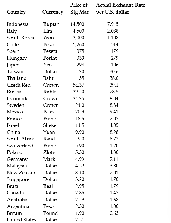
The concept of purchasing power parity or PPP ("the idea that similar foreign and domestic goods … should have the same price in terms of the same currency," Abel, A. and B. Bernanke, Macroeconomics, 4th edition, Boston: Addison Wesley, 476)suggests that the ratio of the Big Mac priced in the local currency to the U.S. dollar price should equal the exchange rate between the two countries.
After entering the data into your spread sheet program, you calculate the predicted exchange rate per U.S. dollar by dividing the price of a Big Mac in local currency by the U.S. price of a Big Mac ($2.51). To test for PPP, you regress the actual exchange rate on the predicted exchange rate.
The estimated regression is as follows: = -27.05 + 1.35 × 1.35×Pr edExRate R2 = 0.994, n = 29, SER = 122.15
(23.74)(0.02)
(a)Your spreadsheet program does not allow you to calculate heteroskedasticity robust standard errors. Instead, the numbers in parenthesis are homoskedasticity only standard errors. State the two null hypothesis under which PPP holds. Should you use a one-tailed or two-tailed alternative hypothesis?
(b)Calculate the two t-statistics.
(c)Using a 5% significance level, what is your decision regarding the null hypothesis given the two t-statistics? What critical values did you use? Are you concerned with the fact that you are testing the two hypothesis sequentially when they are supposed to hold simultaneously?
(d)What assumptions had to be made for you to use Student's t-distribution?
Question
You have obtained measurements of height in inches of 29 female and 81 male students (Studenth)at your university. A regression of the height on a constant and a binary variable (BFemme), which takes a value of one for females and is zero otherwise, yields the following result:  = 71.0 - 4.84×BFemme , R2 = 0.40, SER = 2.0
(0.3)(0.57)
(a)What is the interpretation of the intercept? What is the interpretation of the slope? How tall are females, on average?
(b)Test the hypothesis that females, on average, are shorter than males, at the 1% level.
(c)Is it likely that the error term is homoskedastic here?
= 71.0 - 4.84×BFemme , R2 = 0.40, SER = 2.0(0.3)(0.57)
(a)What is the interpretation of the intercept? What is the interpretation of the slope? How tall are females, on average?
(b)Test the hypothesis that females, on average, are shorter than males, at the 1% level.
(c)Is it likely that the error term is homoskedastic here?
Question
Question
Question
Question
Using data from the Current Population Survey, you estimate the following relationship between average hourly earnings (ahe)and the number of years of education (educ):  = -4.58 + 1.71 educ
The heteroskedasticity-robust standard error on the slope is (0.03). Calculate the 95% confidence interval for the slope. Repeat the exercise using the 90% and then the 99% confidence interval. Can you reject the null hypothesis that the slope coefficient is zero in the population?
= -4.58 + 1.71 educThe heteroskedasticity-robust standard error on the slope is (0.03). Calculate the 95% confidence interval for the slope. Repeat the exercise using the 90% and then the 99% confidence interval. Can you reject the null hypothesis that the slope coefficient is zero in the population?
Question
Question
Question
In a Monte Carlo study, econometricians generate multiple sample regression functions from a known population regression function. For example, the population regression function could be Yi = ?0 + ?1Xi = 100 - 0.5 Xi. The Xs could be generated randomly or, for simplicity, be nonrandom ("fixed over repeated samples"). If we had ten of these Xs, say, and generated twenty Ys, we would obviously always have all observations on a straight line, and the least squares formulae would always return values of 100 and 0.5 numerically. However, if we added an error term, where the errors would be drawn randomly from a normal distribution, say, then the OLS formulae would give us estimates that differed from the population regression function values. Assume you did just that and recorded the values for the slope and the intercept. Then you did the same experiment again (each one of these is called a "replication"). And so forth. After 1,000 replications, you plot the 1,000 intercepts and slopes, and list their summary statistics.
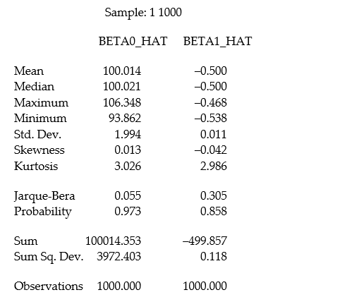
Here are the corresponding graphs: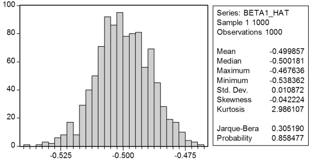
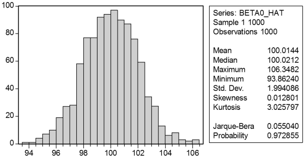 Using the means listed next to the graphs, you see that the averages are not exactly 100 and -0.5. However, they are "close." Test for the difference of these averages from the population values to be statistically significant.
Here are the corresponding graphs:
Using the means listed next to the graphs, you see that the averages are not exactly 100 and -0.5. However, they are "close." Test for the difference of these averages from the population values to be statistically significant. Question
Question
Question
(Requires Appendix material and Calculus)Equation (5.36)in your textbook derives the conditional variance for any old conditionally unbiased estimator 1 to be var( 1  X1, ..., Xn)= where the conditions for conditional unbiasedness are = 0 and = 1. As an alternative to the BLUE proof presented in your textbook, you recall from one of your calculus courses that you could minimize the variance subject to the two constraints, thereby making the variance as small as possible while the constraints are holding. Show that in doing so you get the OLS weights (You may assume that X1,..., Xn are nonrandom (fixed over repeated samples).)
X1, ..., Xn)= where the conditions for conditional unbiasedness are = 0 and = 1. As an alternative to the BLUE proof presented in your textbook, you recall from one of your calculus courses that you could minimize the variance subject to the two constraints, thereby making the variance as small as possible while the constraints are holding. Show that in doing so you get the OLS weights (You may assume that X1,..., Xn are nonrandom (fixed over repeated samples).) Question
Question
Question
Question
Question
Question
Question
Question
Question

Unlock Deck
Sign up to unlock the cards in this deck!
Unlock Deck
Unlock Deck
1/59
Play
Full screen (f)
Deck 5: Regression With a Single Regressor: Hypothesis Tests and Confidence Intervals
1
The p-value for a one-sided left-tail test is given by
A)Pr(Z - tact )= φ(tact).
B)Pr(Z < tact )= φ(tact).
C)Pr(Z < tact )< 1.645.
D)cannot be calculated, since probabilities must always be positive.
A)Pr(Z - tact )= φ(tact).
B)Pr(Z < tact )= φ(tact).
C)Pr(Z < tact )< 1.645.
D)cannot be calculated, since probabilities must always be positive.
B
2
In the presence of heteroskedasticity, and assuming that the usual least squares assumptions hold, the OLS estimator is
A)efficient.
B)BLUE.
C)unbiased and consistent.
D)unbiased but not consistent.
A)efficient.
B)BLUE.
C)unbiased and consistent.
D)unbiased but not consistent.
C
3
If the absolute value of your calculated t-statistic exceeds the critical value from the standard normal distribution, you can
A)reject the null hypothesis.
B)safely assume that your regression results are significant.
C)reject the assumption that the error terms are homoskedastic.
D)conclude that most of the actual values are very close to the regression line.
A)reject the null hypothesis.
B)safely assume that your regression results are significant.
C)reject the assumption that the error terms are homoskedastic.
D)conclude that most of the actual values are very close to the regression line.
A
4
The homoskedasticity-only estimator of the variance of 1 is
A)
B)
C)
D)
A)
B)
C)
D)
Unlock Deck
Unlock for access to all 59 flashcards in this deck.
Unlock Deck
k this deck
5
Finding a small value of the p-value (e.g. less than 5%)
A)indicates evidence in favor of the null hypothesis.
B)implies that the t-statistic is less than 1.96.
C)indicates evidence in against the null hypothesis.
D)will only happen roughly one in twenty samples.
A)indicates evidence in favor of the null hypothesis.
B)implies that the t-statistic is less than 1.96.
C)indicates evidence in against the null hypothesis.
D)will only happen roughly one in twenty samples.
Unlock Deck
Unlock for access to all 59 flashcards in this deck.
Unlock Deck
k this deck
6
Under the least squares assumptions (zero conditional mean for the error term, Xi and Yi being i.i.d., and Xi and ui having finite fourth moments), the OLS estimator for the slope and intercept
A)has an exact normal distribution for n > 15.
B)is BLUE.
C)has a normal distribution even in small samples.
D)is unbiased.
A)has an exact normal distribution for n > 15.
B)is BLUE.
C)has a normal distribution even in small samples.
D)is unbiased.
Unlock Deck
Unlock for access to all 59 flashcards in this deck.
Unlock Deck
k this deck
7
Consider the following regression line: = 698.9 - 2.28 × STR. You are told that the t-statistic on the slope coefficient is 4.38. What is the standard error of the slope coefficient?
A)0.52
B)1.96
C)-1.96
D)4.38
A)0.52
B)1.96
C)-1.96
D)4.38
Unlock Deck
Unlock for access to all 59 flashcards in this deck.
Unlock Deck
k this deck
8
The construction of the t-statistic for a one- and a two-sided hypothesis
A)depends on the critical value from the appropriate distribution.
B)is the same.
C)is different since the critical value must be 1.645 for the one-sided hypothesis, but 1.96 for the two-sided hypothesis (using a 5% probability for the Type I error).
D)uses ±1.96 for the two-sided test, but only +1.96 for the one-sided test.
Unlock Deck
Unlock for access to all 59 flashcards in this deck.
Unlock Deck
k this deck
9
In general, the t-statistic has the following form:
A)
B)
C)
D)
A)
B)
C)
D)
Unlock Deck
Unlock for access to all 59 flashcards in this deck.
Unlock Deck
k this deck
10
When estimating a demand function for a good where quantity demanded is a linear function of the price, you should
A)not include an intercept because the price of the good is never zero.
B)use a one-sided alternative hypothesis to check the influence of price on quantity.
C)use a two-sided alternative hypothesis to check the influence of price on quantity.
D)reject the idea that price determines demand unless the coefficient is at least 1.96.
Unlock Deck
Unlock for access to all 59 flashcards in this deck.
Unlock Deck
k this deck
11
The only difference between a one- and two-sided hypothesis test is
A)the null hypothesis.
B)dependent on the sample size n.
C)the sign of the slope coefficient.
D)how you interpret the t-statistic.
A)the null hypothesis.
B)dependent on the sample size n.
C)the sign of the slope coefficient.
D)how you interpret the t-statistic.
Unlock Deck
Unlock for access to all 59 flashcards in this deck.
Unlock Deck
k this deck
12
With heteroskedastic errors, the weighted least squares estimator is BLUE. You should use OLS with heteroskedasticity-robust standard errors because
A)this method is simpler.
B)the exact form of the conditional variance is rarely known.
C)the Gauss-Markov theorem holds.
D)your spreadsheet program does not have a command for weighted least squares.
A)this method is simpler.
B)the exact form of the conditional variance is rarely known.
C)the Gauss-Markov theorem holds.
D)your spreadsheet program does not have a command for weighted least squares.
Unlock Deck
Unlock for access to all 59 flashcards in this deck.
Unlock Deck
k this deck
13
The proof that OLS is BLUE requires all of the following assumptions with the exception of:
A)the errors are homoskedastic.
B)the errors are normally distributed.
C)E(ui
D)large outliers are unlikely.
A)the errors are homoskedastic.
B)the errors are normally distributed.
C)E(ui
D)large outliers are unlikely.
Unlock Deck
Unlock for access to all 59 flashcards in this deck.
Unlock Deck
k this deck
14
Imagine that you were told that the t-statistic for the slope coefficient of the regression line = 698.9 - 2.28 × STR was 4.38. What are the units of measurement for the t-statistic?
A)points of the test score
B)number of students per teacher
C)
D)standard deviations
A)points of the test score
B)number of students per teacher
C)
D)standard deviations
Unlock Deck
Unlock for access to all 59 flashcards in this deck.
Unlock Deck
k this deck
15
Heteroskedasticity means that
A)homogeneity cannot be assumed automatically for the model.
B)the variance of the error term is not constant.
C)the observed units have different preferences.
D)agents are not all rational.
A)homogeneity cannot be assumed automatically for the model.
B)the variance of the error term is not constant.
C)the observed units have different preferences.
D)agents are not all rational.
Unlock Deck
Unlock for access to all 59 flashcards in this deck.
Unlock Deck
k this deck
16
One of the following steps is not required as a step to test for the null hypothesis:
A)compute the standard error of 1.
B)test for the errors to be normally distributed.
C)compute the t-statistic.
D)compute the p-value.
A)compute the standard error of 1.
B)test for the errors to be normally distributed.
C)compute the t-statistic.
D)compute the p-value.
Unlock Deck
Unlock for access to all 59 flashcards in this deck.
Unlock Deck
k this deck
17
The error term is homoskedastic if
A)var(ui | is constant for i = 1,…, n.
B)var(ui | depends on x.
C)Xi is normally distributed.
D)there are no outliers.
A)var(ui | is constant for i = 1,…, n.
B)var(ui | depends on x.
C)Xi is normally distributed.
D)there are no outliers.
Unlock Deck
Unlock for access to all 59 flashcards in this deck.
Unlock Deck
k this deck
18
A binary variable is often called a
A)dummy variable.
B)dependent variable.
C)residual.
D)power of a test.
A)dummy variable.
B)dependent variable.
C)residual.
D)power of a test.
Unlock Deck
Unlock for access to all 59 flashcards in this deck.
Unlock Deck
k this deck
19
The confidence interval for the sample regression function slope
A)can be used to conduct a test about a hypothesized population regression function slope.
B)can be used to compare the value of the slope relative to that of the intercept.
C)adds and subtracts 1.96 from the slope.
D)allows you to make statements about the economic importance of your estimate.
A)can be used to conduct a test about a hypothesized population regression function slope.
B)can be used to compare the value of the slope relative to that of the intercept.
C)adds and subtracts 1.96 from the slope.
D)allows you to make statements about the economic importance of your estimate.
Unlock Deck
Unlock for access to all 59 flashcards in this deck.
Unlock Deck
k this deck
20
The t-statistic is calculated by dividing
A)the OLS estimator by its standard error.
B)the slope by the standard deviation of the explanatory variable.
C)the estimator minus its hypothesized value by the standard error of the estimator.
D)the slope by 1.96.
A)the OLS estimator by its standard error.
B)the slope by the standard deviation of the explanatory variable.
C)the estimator minus its hypothesized value by the standard error of the estimator.
D)the slope by 1.96.
Unlock Deck
Unlock for access to all 59 flashcards in this deck.
Unlock Deck
k this deck
21
You extract approximately 5,000 observations from the Current Population Survey (CPS)and estimate the following regression function: = 3.32 - 0.45 Age, R2= 0.02, SER = 8.66 (1.00)(0.04)
Where ahe is average hourly earnings, and Age is the individual's age. Given the specification, your 95% confidence interval for the effect of changing age by 5 years is approximately
A)[$1.96, $2.54]
B)[$2.32, $4.32]
C)[$1.35, $5.30]
D)cannot be determined given the information provided
Where ahe is average hourly earnings, and Age is the individual's age. Given the specification, your 95% confidence interval for the effect of changing age by 5 years is approximately
A)[$1.96, $2.54]
B)[$2.32, $4.32]
C)[$1.35, $5.30]
D)cannot be determined given the information provided
Unlock Deck
Unlock for access to all 59 flashcards in this deck.
Unlock Deck
k this deck
22
You have collected 14,925 observations from the Current Population Survey. There are 6,285 females in the sample, and 8,640 males. The females report a mean of average hourly earnings of $16.50 with a standard deviation of $9.06. The males have an average of $20.09 and a standard deviation of $10.85. The overall mean average hourly earnings is $18.58.
a. Using the t-statistic for testing differences between two means (section 3.4 of your textbook), decide whether or not there is sufficient evidence to reject the null hypothesis that females and males have identical average hourly earnings.
b. You decide to run two regressions: first, you simply regress average hourly earnings on an intercept only. Next, you repeat this regression, but only for the 6,285 females in the sample. What will the regression coefficients be in each of the two regressions?
c. Finally you run a regression over the entire sample of average hourly earnings on an intercept and a binary variable DFemme, where this variable takes on a value of 1 if the individual is a female, and is 0 otherwise. What will be the value of the intercept? What will be the value of the coefficient of the binary variable?
d. What is the standard error on the slope coefficient? What is the t-statistic?
e. Had you used the homoskedasticity-only standard error in (d)and calculated the t-statistic, how would you have had to change the test-statistic in (a)to get the identical result?
Unlock Deck
Unlock for access to all 59 flashcards in this deck.
Unlock Deck
k this deck
23
If the errors are heteroskedastic, then
A)OLS is BLUE.
B)WLS is BLUE if the conditional variance of the errors is known up to a constant factor of proportionality.
C)LAD is BLUE if the conditional variance of the errors is known up to a constant factor of proportionality.
D)OLS is efficient.
A)OLS is BLUE.
B)WLS is BLUE if the conditional variance of the errors is known up to a constant factor of proportionality.
C)LAD is BLUE if the conditional variance of the errors is known up to a constant factor of proportionality.
D)OLS is efficient.
Unlock Deck
Unlock for access to all 59 flashcards in this deck.
Unlock Deck
k this deck
24
In order to formulate whether or not the alternative hypothesis is one-sided or two-sided, you need some guidance from economic theory. Choose at least three examples from economics or other fields where you have a clear idea what the null hypothesis and the alternative hypothesis for the slope coefficient should be. Write a brief justification for your answer.
Unlock Deck
Unlock for access to all 59 flashcards in this deck.
Unlock Deck
k this deck
25
Explain carefully the relationship between a confidence interval, a one-sided hypothesis test, and a two-sided hypothesis test. What is the unit of measurement of the t-statistic?
Unlock Deck
Unlock for access to all 59 flashcards in this deck.
Unlock Deck
k this deck
26
Carefully discuss the advantages of using heteroskedasticity-robust standard errors over standard errors calculated under the assumption of homoskedasticity. Give at least five examples where it is very plausible to assume that the errors display heteroskedasticity.
Unlock Deck
Unlock for access to all 59 flashcards in this deck.
Unlock Deck
k this deck
27
(Requires Appendix material from Chapters 4 and 5)Shortly before you are making a group presentation on the testscore/student-teacher ratio results, you realize that one of your peers forgot to type all the relevant information on one of your slides. Here is what you see: = 698.9 - STR, R2 = 0.051, SER = 18.6
(9.47)(0.48)
In addition, your group member explains that he ran the regression in a standard spreadsheet program, and that, as a result, the standard errors in parenthesis are homoskedasticity-only standard errors.
(a)Find the value for the slope coefficient.
(b)Calculate the t-statistic for the slope and the intercept. Test the hypothesis that the intercept and the slope are different from zero.
(c)Should you be concerned that your group member only gave you the result for the homoskedasticity-only standard error formula, instead of using the heteroskedasticity-robust standard errors?
Unlock Deck
Unlock for access to all 59 flashcards in this deck.
Unlock Deck
k this deck
28
Consider the estimated equation from your textbook =698.9 - 2.28 STR, R2 = 0.051, SER = 18.6 (10.4)(0.52)
The t-statistic for the slope is approximately
A)4.38
B)67.20
C)0.52
D)1.76
The t-statistic for the slope is approximately
A)4.38
B)67.20
C)0.52
D)1.76
Unlock Deck
Unlock for access to all 59 flashcards in this deck.
Unlock Deck
k this deck
29
(Continuation from Chapter 4, number 6)The neoclassical growth model predicts that for identical savings rates and population growth rates, countries should converge to the per capita income level. This is referred to as the convergence hypothesis. One way to test for the presence of convergence is to compare the growth rates over time to the initial starting level.
(a)The results of the regression for 104 countries were as follows: = 0.019 - 0.0006 × RelProd60, R2= 0.00007, SER = 0.016
(0.004)(0.0073) where g6090 is the average annual growth rate of GDP per worker for the 1960-1990 sample period, and RelProd60 is GDP per worker relative to the United States in 1960. Numbers in parenthesis are heteroskedasticity robust standard errors.
Using the OLS estimator with homoskedasticity-only standard errors, the results changed as follows: = 0.019 - 0.0006×RelProd60, R2= 0.00007, SER = 0.016
(0.002)(0.0068)
Why didn't the estimated coefficients change? Given that the standard error of the slope is now smaller, can you reject the null hypothesis of no beta convergence? Are the results in the second equation more reliable than the results in the first equation? Explain.
(b)You decide to restrict yourself to the 24 OECD countries in the sample. This changes your regression output as follows (numbers in parenthesis are heteroskedasticity robust standard errors): = 0.048 - 0.0404 RelProd60, R2 = 0.82, SER = 0.0046
(0.004)(0.0063)
Test for evidence of convergence now. If your conclusion is different than in (a), speculate why this is the case.
(c)The authors of your textbook have informed you that unless you have more than 100 observations, it may not be plausible to assume that the distribution of your OLS estimators is normal. What are the implications here for testing the significance of your theory?
(a)The results of the regression for 104 countries were as follows: = 0.019 - 0.0006 × RelProd60, R2= 0.00007, SER = 0.016
(0.004)(0.0073)
where g6090 is the average annual growth rate of GDP per worker for the 1960-1990 sample period, and RelProd60 is GDP per worker relative to the United States in 1960. Numbers in parenthesis are heteroskedasticity robust standard errors.Using the OLS estimator with homoskedasticity-only standard errors, the results changed as follows: = 0.019 - 0.0006×RelProd60, R2= 0.00007, SER = 0.016
(0.002)(0.0068)
Why didn't the estimated coefficients change? Given that the standard error of the slope is now smaller, can you reject the null hypothesis of no beta convergence? Are the results in the second equation more reliable than the results in the first equation? Explain.
(b)You decide to restrict yourself to the 24 OECD countries in the sample. This changes your regression output as follows (numbers in parenthesis are heteroskedasticity robust standard errors): = 0.048 - 0.0404 RelProd60, R2 = 0.82, SER = 0.0046
(0.004)(0.0063)
Test for evidence of convergence now. If your conclusion is different than in (a), speculate why this is the case.
(c)The authors of your textbook have informed you that unless you have more than 100 observations, it may not be plausible to assume that the distribution of your OLS estimators is normal. What are the implications here for testing the significance of your theory?
Unlock Deck
Unlock for access to all 59 flashcards in this deck.
Unlock Deck
k this deck
30
(Continuation from Chapter 4)At a recent county fair, you observed that at one stand people's weight was forecasted, and were surprised by the accuracy (within a range). Thinking about how the person could have predicted your weight fairly accurately (despite the fact that she did not know about your "heavy bones"), you think about how this could have been accomplished. You remember that medical charts for children contain 5%, 25%, 50%, 75% and 95% lines for a weight/height relationship and decide to conduct an experiment with 110 of your peers. You collect the data and calculate the following sums: where the height is measured in inches and weight in pounds. (Small letters refer to deviations from means as in zi = Zi - )
(a)Calculate the homoskedasticity-only standard errors and, using the resulting t-statistic, perform a test on the null hypothesis that there is no relationship between height and weight in the population of college students.
(b)What is the alternative hypothesis in the above test, and what level of significance did you choose?
(c)Statistics and econometrics textbooks often ask you to calculate critical values based on some level of significance, say 1%, 5%, or 10%. What sort of criteria do you think should play a role in determining which level of significance to choose?
(d)What do you think the relationship is between testing for the significance of the slope and whether or not the regression R2 is zero?
Unlock Deck
Unlock for access to all 59 flashcards in this deck.
Unlock Deck
k this deck
31
Using the textbook example of 420 California school districts and the regression of testscores on the student-teacher ratio, you find that the standard error on the slope coefficient is 0.51 when using the heteroskedasticity robust formula, while it is 0.48 when employing the homoskedasticity only formula. When calculating the t-statistic, the recommended procedure is to
A)use the homoskedasticity only formula because the t-statistic becomes larger
B)first test for homoskedasticity of the errors and then make a decision
C)use the heteroskedasticity robust formula
D)make a decision depending on how much different the estimate of the slope is under the two procedures
A)use the homoskedasticity only formula because the t-statistic becomes larger
B)first test for homoskedasticity of the errors and then make a decision
C)use the heteroskedasticity robust formula
D)make a decision depending on how much different the estimate of the slope is under the two procedures
Unlock Deck
Unlock for access to all 59 flashcards in this deck.
Unlock Deck
k this deck
32
The homoskedastic normal regression assumptions are all of the following with the exception of:
A)the errors are homoskedastic.
B)the errors are normally distributed.
C)there are no outliers.
D)there are at least 10 observations.
A)the errors are homoskedastic.
B)the errors are normally distributed.
C)there are no outliers.
D)there are at least 10 observations.
Unlock Deck
Unlock for access to all 59 flashcards in this deck.
Unlock Deck
k this deck
33
Using 143 observations, assume that you had estimated a simple regression function and that your estimate for the slope was 0.04, with a standard error of 0.01. You want to test whether or not the estimate is statistically significant. Which of the following possible decisions is the only correct one:
A)you decide that the coefficient is small and hence most likely is zero in the population
B)the slope is statistically significant since it is four standard errors away from zero
C)the response of Y given a change in X must be economically important since it is statistically significant
D)since the slope is very small, so must be the regression R2.
Unlock Deck
Unlock for access to all 59 flashcards in this deck.
Unlock Deck
k this deck
34
(Continuation from Chapter 4, number 5)You have learned in one of your economics courses that one of the determinants of per capita income (the "Wealth of Nations")is the population growth rate. Furthermore you also found out that the Penn World Tables contain income and population data for 104 countries of the world. To test this theory, you regress the GDP per worker (relative to the United States)in 1990 (RelPersInc)on the difference between the average population growth rate of that country (n)to the U.S. average population growth rate (nus )for the years 1980 to 1990. This results in the following regression output: = 0.518 - 18.831×(n - nus), R2=0.522, SER = 0.197
(0.056)(3.177)
(a)Is there any reason to believe that the variance of the error terms is homoskedastic?
(b)Is the relationship statistically significant?
= 0.518 - 18.831×(n - nus), R2=0.522, SER = 0.197(0.056)(3.177)
(a)Is there any reason to believe that the variance of the error terms is homoskedastic?
(b)Is the relationship statistically significant?
Unlock Deck
Unlock for access to all 59 flashcards in this deck.
Unlock Deck
k this deck
35
(Continuation from Chapter 4)Sir Francis Galton, a cousin of James Darwin, examined the relationship between the height of children and their parents towards the end of the 19th century. It is from this study that the name "regression" originated. You decide to update his findings by collecting data from 110 college students, and estimate the following relationship: = 19.6 + 0.73 × Midparh, R2 = 0.45, SER = 2.0
(7.2)(0.10)
where Studenth is the height of students in inches, and Midparh is the average of the parental heights. Values in parentheses are heteroskedasticity robust standard errors. (Following Galton's methodology, both variables were adjusted so that the average female height was equal to the average male height.)
(a)Test for the statistical significance of the slope coefficient.
(b)If children, on average, were expected to be of the same height as their parents, then this would imply two hypotheses, one for the slope and one for the intercept.
(i)What should the null hypothesis be for the intercept? Calculate the relevant t-statistic and carry out the hypothesis test at the 1% level.
(ii)What should the null hypothesis be for the slope? Calculate the relevant t-statistic and carry out the hypothesis test at the 5% level.
(c)Can you reject the null hypothesis that the regression R2 is zero?
(d)Construct a 95% confidence interval for a one inch increase in the average of parental height.
= 19.6 + 0.73 × Midparh, R2 = 0.45, SER = 2.0(7.2)(0.10)
where Studenth is the height of students in inches, and Midparh is the average of the parental heights. Values in parentheses are heteroskedasticity robust standard errors. (Following Galton's methodology, both variables were adjusted so that the average female height was equal to the average male height.)
(a)Test for the statistical significance of the slope coefficient.
(b)If children, on average, were expected to be of the same height as their parents, then this would imply two hypotheses, one for the slope and one for the intercept.
(i)What should the null hypothesis be for the intercept? Calculate the relevant t-statistic and carry out the hypothesis test at the 1% level.
(ii)What should the null hypothesis be for the slope? Calculate the relevant t-statistic and carry out the hypothesis test at the 5% level.
(c)Can you reject the null hypothesis that the regression R2 is zero?
(d)Construct a 95% confidence interval for a one inch increase in the average of parental height.
Unlock Deck
Unlock for access to all 59 flashcards in this deck.
Unlock Deck
k this deck
36
You have collected data for the 50 U.S. states and estimated the following relationship between the change in the unemployment rate from the previous year ( )and the growth rate of the respective state real GDP (gy). The results are as follows = 2.81 - 0.23 gy, R2= 0.36, SER = 0.78 (0.12)(0.04)
Assuming that the estimator has a normal distribution, the 95% confidence interval for the slope is approximately the interval
A)[2.57, 3.05]
B)[-0.31,0.15]
C)[-0.31, -0.15]
D)[-0.33, -0.13]
Assuming that the estimator has a normal distribution, the 95% confidence interval for the slope is approximately the interval
A)[2.57, 3.05]
B)[-0.31,0.15]
C)[-0.31, -0.15]
D)[-0.33, -0.13]
Unlock Deck
Unlock for access to all 59 flashcards in this deck.
Unlock Deck
k this deck
37
You recall from one of your earlier lectures in macroeconomics that the per capita income depends on the savings rate of the country: those who save more end up with a higher standard of living. To test this theory, you collect data from the Penn World Tables on GDP per worker relative to the United States (RelProd)in 1990 and the average investment share of GDP from 1980-1990 (SK), remembering that investment equals saving. The regression results in the following output: = -0.08 + 2.44×SK, R2=0.46, SER = 0.21
(0.04)(0.38)
(a)Interpret the regression results carefully.
(b)Calculate the t-statistics to determine whether the two coefficients are significantly different from zero. Justify the use of a one-sided or two-sided test.
(c)You accidentally forget to use the heteroskedasticity-robust standard errors option in your regression package and estimate the equation using homoskedasticity-only standard errors. This changes the results as follows: = -0.08 + 2.44×SK, R2=0.46, SER = 0.21
(0.04)(0.26)
You are delighted to find that the coefficients have not changed at all and that your results have become even more significant. Why haven't the coefficients changed? Are the results really more significant? Explain.
(d)Upon reflection you think about the advantages of OLS with and without homoskedasticity-only standard errors. What are these advantages? Is it likely that the error terms would be heteroskedastic in this situation?
= -0.08 + 2.44×SK, R2=0.46, SER = 0.21(0.04)(0.38)
(a)Interpret the regression results carefully.
(b)Calculate the t-statistics to determine whether the two coefficients are significantly different from zero. Justify the use of a one-sided or two-sided test.
(c)You accidentally forget to use the heteroskedasticity-robust standard errors option in your regression package and estimate the equation using homoskedasticity-only standard errors. This changes the results as follows:
= -0.08 + 2.44×SK, R2=0.46, SER = 0.21(0.04)(0.26)
You are delighted to find that the coefficients have not changed at all and that your results have become even more significant. Why haven't the coefficients changed? Are the results really more significant? Explain.
(d)Upon reflection you think about the advantages of OLS with and without homoskedasticity-only standard errors. What are these advantages? Is it likely that the error terms would be heteroskedastic in this situation?
Unlock Deck
Unlock for access to all 59 flashcards in this deck.
Unlock Deck
k this deck
38
(continuation from Chapter 4, number 3)You have obtained a sub-sample of 1744 individuals from the Current Population Survey (CPS)and are interested in the relationship between weekly earnings and age. The regression, using heteroskedasticity-robust standard errors, yielded the following result: = 239.16 + 5.20×Age , R2 = 0.05, SER = 287.21.,
(20.24)(0.57)
where Earn and Age are measured in dollars and years respectively.
(a)Is the relationship between Age and Earn statistically significant?
(b)The variance of the error term and the variance of the dependent variable are related. Given the distribution of earnings, do you think it is plausible that the distribution of errors is normal?
(c)Construct a 95% confidence interval for both the slope and the intercept.
= 239.16 + 5.20×Age , R2 = 0.05, SER = 287.21.,(20.24)(0.57)
where Earn and Age are measured in dollars and years respectively.
(a)Is the relationship between Age and Earn statistically significant?
(b)The variance of the error term and the variance of the dependent variable are related. Given the distribution of earnings, do you think it is plausible that the distribution of errors is normal?
(c)Construct a 95% confidence interval for both the slope and the intercept.
Unlock Deck
Unlock for access to all 59 flashcards in this deck.
Unlock Deck
k this deck
39
(Continuation of the Purchasing Power Parity question from Chapter 4)The news-magazine The Economist regularly publishes data on the so called Big Mac index and exchange rates between countries. The data for 30 countries from the April 29, 2000 issue is listed below:
The concept of purchasing power parity or PPP ("the idea that similar foreign and domestic goods … should have the same price in terms of the same currency," Abel, A. and B. Bernanke, Macroeconomics, 4th edition, Boston: Addison Wesley, 476)suggests that the ratio of the Big Mac priced in the local currency to the U.S. dollar price should equal the exchange rate between the two countries.
After entering the data into your spread sheet program, you calculate the predicted exchange rate per U.S. dollar by dividing the price of a Big Mac in local currency by the U.S. price of a Big Mac ($2.51). To test for PPP, you regress the actual exchange rate on the predicted exchange rate.
The estimated regression is as follows: = -27.05 + 1.35 × 1.35×Pr edExRate R2 = 0.994, n = 29, SER = 122.15
(23.74)(0.02)
(a)Your spreadsheet program does not allow you to calculate heteroskedasticity robust standard errors. Instead, the numbers in parenthesis are homoskedasticity only standard errors. State the two null hypothesis under which PPP holds. Should you use a one-tailed or two-tailed alternative hypothesis?
(b)Calculate the two t-statistics.
(c)Using a 5% significance level, what is your decision regarding the null hypothesis given the two t-statistics? What critical values did you use? Are you concerned with the fact that you are testing the two hypothesis sequentially when they are supposed to hold simultaneously?
(d)What assumptions had to be made for you to use Student's t-distribution?
Unlock Deck
Unlock for access to all 59 flashcards in this deck.
Unlock Deck
k this deck
40
You have obtained measurements of height in inches of 29 female and 81 male students (Studenth)at your university. A regression of the height on a constant and a binary variable (BFemme), which takes a value of one for females and is zero otherwise, yields the following result: = 71.0 - 4.84×BFemme , R2 = 0.40, SER = 2.0
(0.3)(0.57)
(a)What is the interpretation of the intercept? What is the interpretation of the slope? How tall are females, on average?
(b)Test the hypothesis that females, on average, are shorter than males, at the 1% level.
(c)Is it likely that the error term is homoskedastic here?
= 71.0 - 4.84×BFemme , R2 = 0.40, SER = 2.0(0.3)(0.57)
(a)What is the interpretation of the intercept? What is the interpretation of the slope? How tall are females, on average?
(b)Test the hypothesis that females, on average, are shorter than males, at the 1% level.
(c)Is it likely that the error term is homoskedastic here?
Unlock Deck
Unlock for access to all 59 flashcards in this deck.
Unlock Deck
k this deck
41
The effect of decreasing the student-teacher ratio by one is estimated to result in an improvement of the districtwide score by 2.28 with a standard error of 0.52. Construct a 90% and 99% confidence interval for the size of the slope coefficient and the corresponding predicted effect of changing the student-teacher ratio by one. What is the intuition on why the 99% confidence interval is wider than the 90% confidence interval?
Unlock Deck
Unlock for access to all 59 flashcards in this deck.
Unlock Deck
k this deck
42
Using the California School data set from your textbook, you run the following regression: = 698.9 - 2.28 STR
n = 420, R2 = 0.051, SER = 18.6
where TestScore is the average test score in the district and STR is the student-teacher ratio. Using heteroskedasticity robust standard errors, you find while choosing the homoskedasticity-only option, the standard error is 0.48.
a. Calculate the t-statistic for both standard errors.
b. Which of the two t-statistics should you base your inference on?
Unlock Deck
Unlock for access to all 59 flashcards in this deck.
Unlock Deck
k this deck
43
In many of the cases discussed in your textbook, you test for the significance of the slope at the 5% level. What is the size of the test? What is the power of the test? Why is the probability of committing a Type II error so large here?
Unlock Deck
Unlock for access to all 59 flashcards in this deck.
Unlock Deck
k this deck
44
Using data from the Current Population Survey, you estimate the following relationship between average hourly earnings (ahe)and the number of years of education (educ): = -4.58 + 1.71 educ
The heteroskedasticity-robust standard error on the slope is (0.03). Calculate the 95% confidence interval for the slope. Repeat the exercise using the 90% and then the 99% confidence interval. Can you reject the null hypothesis that the slope coefficient is zero in the population?
= -4.58 + 1.71 educThe heteroskedasticity-robust standard error on the slope is (0.03). Calculate the 95% confidence interval for the slope. Repeat the exercise using the 90% and then the 99% confidence interval. Can you reject the null hypothesis that the slope coefficient is zero in the population?
Unlock Deck
Unlock for access to all 59 flashcards in this deck.
Unlock Deck
k this deck
45
Assume that the homoskedastic normal regression assumption hold. Using the Student t-distribution, find the critical value for the following situation:
(a)n = 28, 5% significance level, one-sided test.
(b)n = 40, 1% significance level, two-sided test.
(c)n = 10, 10% significance level, one-sided test.
(d)n = ∞, 5% significance level, two-sided test.
(a)n = 28, 5% significance level, one-sided test.
(b)n = 40, 1% significance level, two-sided test.
(c)n = 10, 10% significance level, one-sided test.
(d)n = ∞, 5% significance level, two-sided test.
Unlock Deck
Unlock for access to all 59 flashcards in this deck.
Unlock Deck
k this deck
46
Using the California School data set from your textbook, you run the following regression: = 698.9 - 2.28 STR
n = 420, SER = 9.4
where TestScore is the average test score in the district and STR is the student-teacher ratio. The sample standard deviation of test scores is 19.05, and the sample standard deviation of the student teacher ratio is 1.89.
a.
Find the regression R2 and the correlation coefficient between test scores and the student teacher ratio.
b.
Find the homoskedasticity-only standard error of the slope.
Unlock Deck
Unlock for access to all 59 flashcards in this deck.
Unlock Deck
k this deck
47
In a Monte Carlo study, econometricians generate multiple sample regression functions from a known population regression function. For example, the population regression function could be Yi = ?0 + ?1Xi = 100 - 0.5 Xi. The Xs could be generated randomly or, for simplicity, be nonrandom ("fixed over repeated samples"). If we had ten of these Xs, say, and generated twenty Ys, we would obviously always have all observations on a straight line, and the least squares formulae would always return values of 100 and 0.5 numerically. However, if we added an error term, where the errors would be drawn randomly from a normal distribution, say, then the OLS formulae would give us estimates that differed from the population regression function values. Assume you did just that and recorded the values for the slope and the intercept. Then you did the same experiment again (each one of these is called a "replication"). And so forth. After 1,000 replications, you plot the 1,000 intercepts and slopes, and list their summary statistics.
Here are the corresponding graphs: Using the means listed next to the graphs, you see that the averages are not exactly 100 and -0.5. However, they are "close." Test for the difference of these averages from the population values to be statistically significant.
Here are the corresponding graphs:
Using the means listed next to the graphs, you see that the averages are not exactly 100 and -0.5. However, they are "close." Test for the difference of these averages from the population values to be statistically significant. Unlock Deck
Unlock for access to all 59 flashcards in this deck.
Unlock Deck
k this deck
48
The neoclassical growth model predicts that for identical savings rates and population growth rates, countries should converge to the per capita income level. This is referred to as the convergence hypothesis. One way to test for the presence of convergence is to compare the growth rates over time to the initial starting level, i.e., to run the regression = + × RelProd60 , where g6090 is the average annual growth rate of GDP per worker for the 1960-1990 sample period, and RelProd60 is GDP per worker relative to the United States in 1960. Under the null hypothesis of no convergence, ?1 = 0; H1 : ?1 < 0, implying ("beta")convergence. Using a standard regression package, you get the following output:
Dependent Variable: G6090
Method: Least Squares
Date: 07/11/06 Time: 05:46
Sample: 1 104
Included observations: 104
White Heteroskedasticity-Consistent Standard Errors & Covariance
You are delighted to see that this program has already calculated p-values for you. However, a peer of yours points out that the correct p-value should be 0.4562. Who is right?
Unlock Deck
Unlock for access to all 59 flashcards in this deck.
Unlock Deck
k this deck
49
Your textbook discussed the regression model when X is a binary variable
Yi = ?0 + ?1Di + ui, i = 1..., n
Let Y represent wages, and let D be one for females, and 0 for males. Using the OLS formula for the slope coefficient, prove that is the difference between the average wage for males and the average wage for females.
Yi = ?0 + ?1Di + ui, i = 1..., n
Let Y represent wages, and let D be one for females, and 0 for males. Using the OLS formula for the slope coefficient, prove that is the difference between the average wage for males and the average wage for females.
Unlock Deck
Unlock for access to all 59 flashcards in this deck.
Unlock Deck
k this deck
50
(Requires Appendix material and Calculus)Equation (5.36)in your textbook derives the conditional variance for any old conditionally unbiased estimator 1 to be var( 1 X1, ..., Xn)= where the conditions for conditional unbiasedness are = 0 and = 1. As an alternative to the BLUE proof presented in your textbook, you recall from one of your calculus courses that you could minimize the variance subject to the two constraints, thereby making the variance as small as possible while the constraints are holding. Show that in doing so you get the OLS weights (You may assume that X1,..., Xn are nonrandom (fixed over repeated samples).)
X1, ..., Xn)= where the conditions for conditional unbiasedness are = 0 and = 1. As an alternative to the BLUE proof presented in your textbook, you recall from one of your calculus courses that you could minimize the variance subject to the two constraints, thereby making the variance as small as possible while the constraints are holding. Show that in doing so you get the OLS weights (You may assume that X1,..., Xn are nonrandom (fixed over repeated samples).) Unlock Deck
Unlock for access to all 59 flashcards in this deck.
Unlock Deck
k this deck
51
Consider the following two models involving binary variables as explanatory variables: = + DFemme and = DFemme + Male
where Wage is the hourly wage rate, DFemme is a binary variable that is equal to 1 if the person is a female, and 0 if the person is a male. Male = 1 - DFemme. Even though you have not learned about regression functions with two explanatory variables (or regressions without an intercept), assume that you had estimated both models, i.e., you obtained the estimates for the regression coefficients.
What is the predicted wage for a male in the two models? What is the predicted wage for a female in the two models? What is the relationship between the ? s and the ?s? Why would you prefer one model over the other?
Unlock Deck
Unlock for access to all 59 flashcards in this deck.
Unlock Deck
k this deck
52
Assume that your population regression function is
Yi = ?iXi + ui
i.e., a regression through the origin (no intercept). Under the homoskedastic normal regression assumptions, the t-statistic will have a Student t distribution with n-1 degrees of freedom, not n-2 degrees of freedom, as was the case in Chapter 5 of your textbook. Explain. Do you think that the residuals will still sum to zero for this case?
Unlock Deck
Unlock for access to all 59 flashcards in this deck.
Unlock Deck
k this deck
53
(Requires Appendix material)Your textbook shows that OLS is a linear estimator 1 = , where For OLS to be conditionally unbiased, the following two conditions must hold: and = 1. Show that this is the case.
Unlock Deck
Unlock for access to all 59 flashcards in this deck.
Unlock Deck
k this deck
54
Let be distributed N(0, ), i.e., the errors are distributed normally with a constant variance (homoskedasticity). This results in being distributed N(?1, ), where Statistical inference would be straightforward if was known. One way to deal with this problem is to replace with an estimator Clearly since this introduces more uncertainty, you cannot expect to be still normally distributed. Indeed, the t-statistic now follows Student's t distribution. Look at the table for the Student t-distribution and focus on the 5% two-sided significance level. List the critical values for 10 degrees of freedom, 30 degrees of freedom, 60 degrees of freedom, and finally ? degrees of freedom. Describe how the notion of uncertainty about can be incorporated about the tails of the t-distribution as the degrees of freedom increase.
Unlock Deck
Unlock for access to all 59 flashcards in this deck.
Unlock Deck
k this deck
55
Changing the units of measurement obviously will have an effect on the slope of your regression function. For example, let Y*= aY and X* = bX. Then it is easy but tedious to show that Given this result, how do you think the standard errors and the regression R2 will change?
Unlock Deck
Unlock for access to all 59 flashcards in this deck.
Unlock Deck
k this deck
56
Consider the sample regression function i = + Xi. The table below lists estimates for the slope ( )and the variance of the slope estimator ( ). In each case calculate the p-value for the null hypothesis of ?1 = 0 and a two-tailed alternative hypothesis. Indicate in which case you would reject the null hypothesis at the 5% significance level.
Unlock Deck
Unlock for access to all 59 flashcards in this deck.
Unlock Deck
k this deck
57
Below you are asked to decide on whether or not to use a one-sided alternative or a two-sided alternative hypothesis for the slope coefficient. Briefly justify your decision.
(a) = 0 + 1pi, where qd is the quantity demanded for a good, and p is its price.
(b) = 0 + 1
, where is the actual house price, and is the assessed house price. You want to test whether or not the assessment is correct, on average.
(c) i = 0 + 1
, where C is household consumption, and Yd is personal disposable income.
Unlock Deck
Unlock for access to all 59 flashcards in this deck.
Unlock Deck
k this deck
58
Your textbook discussed the regression model when X is a binary variable
Yi = ?0 + ?iDi + ui, i = 1,..., n
Let Y represent wages, and let D be one for females, and 0 for males. Using the OLS formula for the intercept coefficient, prove that is the average wage for males.
Yi = ?0 + ?iDi + ui, i = 1,..., n
Let Y represent wages, and let D be one for females, and 0 for males. Using the OLS formula for the intercept coefficient, prove that is the average wage for males.
Unlock Deck
Unlock for access to all 59 flashcards in this deck.
Unlock Deck
k this deck
59
Your textbook states that under certain restrictive conditions, the t- statistic has a Student t-distribution with n-2 degrees of freedom. The loss of two degrees of freedom is the result of OLS forcing two restrictions onto the data. What are these two conditions, and when did you impose them onto the data set in your derivation of the OLS estimator?
Unlock Deck
Unlock for access to all 59 flashcards in this deck.
Unlock Deck
k this deck
Unlock Deck
Unlock for access to all 59 flashcards in this deck.


