Exam 5: Regression With a Single Regressor: Hypothesis Tests and Confidence Intervals

The p-value for a one-sided left-tail test is given by

Finding a small value of the p-value (e.g. less than 5%)

Assume that the homoskedastic normal regression assumption hold. Using the Student t-distribution, find the critical value for the following situation: (a)n = 28, 5% significance level, one-sided test. (b)n = 40, 1% significance level, two-sided test. (c)n = 10, 10% significance level, one-sided test. (d)n = ∞, 5% significance level, two-sided test.

With heteroskedastic errors, the weighted least squares estimator is BLUE. You should use OLS with heteroskedasticity-robust standard errors because

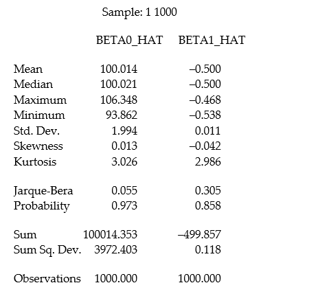
In a Monte Carlo study, econometricians generate multiple sample regression functions from a known population regression function. For example, the population regression function could be Y_i = ?₀ + ?₁X_i = 100 - 0.5 X_i. The Xs could be generated randomly or, for simplicity, be nonrandom ("fixed over repeated samples"). If we had ten of these Xs, say, and generated twenty Ys, we would obviously always have all observations on a straight line, and the least squares formulae would always return values of 100 and 0.5 numerically. However, if we added an error term, where the errors would be drawn randomly from a normal distribution, say, then the OLS formulae would give us estimates that differed from the population regression function values. Assume you did just that and recorded the values for the slope and the intercept. Then you did the same experiment again (each one of these is called a "replication"). And so forth. After 1,000 replications, you plot the 1,000 intercepts and slopes, and list their summary statistics. 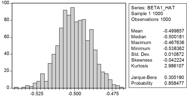Here are the corresponding graphs: 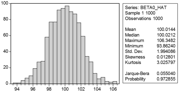Using the means listed next to the graphs, you see that the averages are not exactly 100 and -0.5. However, they are "close." Test for the difference of these averages from the population values to be statistically significant.

Carefully discuss the advantages of using heteroskedasticity-robust standard errors over standard errors calculated under the assumption of homoskedasticity. Give at least five examples where it is very plausible to assume that the errors display heteroskedasticity.

Using the textbook example of 420 California school districts and the regression of testscores on the student-teacher ratio, you find that the standard error on the slope coefficient is 0.51 when using the heteroskedasticity robust formula, while it is 0.48 when employing the homoskedasticity only formula. When calculating the t-statistic, the recommended procedure is to

Under the least squares assumptions (zero conditional mean for the error term, X_i and Y_i being i.i.d., and X_i and u_i having finite fourth moments), the OLS estimator for the slope and intercept

In the presence of heteroskedasticity, and assuming that the usual least squares assumptions hold, the OLS estimator is

(Requires Appendix material from Chapters 4 and 5)Shortly before you are making a group presentation on the testscore/student-teacher ratio results, you realize that one of your peers forgot to type all the relevant information on one of your slides. Here is what you see: $\widehat {\\text { TestScore }}$ = 698.9 - STR, R² = 0.051, SER = 18.6 (9.47)(0.48) In addition, your group member explains that he ran the regression in a standard spreadsheet program, and that, as a result, the standard errors in parenthesis are homoskedasticity-only standard errors. (a)Find the value for the slope coefficient. (b)Calculate the t-statistic for the slope and the intercept. Test the hypothesis that the intercept and the slope are different from zero. (c)Should you be concerned that your group member only gave you the result for the homoskedasticity-only standard error formula, instead of using the heteroskedasticity-robust standard errors?

Your textbook discussed the regression model when X is a binary variable Y_i = ?₀ + ?₁D_i + u_i, i = 1..., n Let Y represent wages, and let D be one for females, and 0 for males. Using the OLS formula for the slope coefficient, prove that $\hat{\beta}_ { 1 }$ is the difference between the average wage for males and the average wage for females.

The proof that OLS is BLUE requires all of the following assumptions with the exception of:

Explain carefully the relationship between a confidence interval, a one-sided hypothesis test, and a two-sided hypothesis test. What is the unit of measurement of the t-statistic?

The neoclassical growth model predicts that for identical savings rates and population growth rates, countries should converge to the per capita income level. This is referred to as the convergence hypothesis. One way to test for the presence of convergence is to compare the growth rates over time to the initial starting level, i.e., to run the regression $\widehat { g 6090 }$ = $\widehat { \beta 0 }$ + $\widehat { \beta 1 }$ × RelProd₆₀ , where g6090 is the average annual growth rate of GDP per worker for the 1960-1990 sample period, and RelProd₆₀ is GDP per worker relative to the United States in 1960. Under the null hypothesis of no convergence, ?₁ = 0; H₁ : ?₁ < 0, implying ("beta")convergence. Using a standard regression package, you get the following output: Dependent Variable: G6090 Method: Least Squares Date: 07/11/06 Time: 05:46 Sample: 1 104 Included observations: 104 White Heteroskedasticity-Consistent Standard Errors & Covariance Variable Coefficient Std. Error t-Statistic Prob. C 0.018989 0.002392 7.939864 0.0000 YL60 -0.000566 0.005056 -0.111948 0.9111 R-squared 0.000068 Mean dependent var 0.018846 Adjusted R-squared -0.009735 S.D. dependent var 0.015915 S.E. of regression 0.015992 Akaike info criterion -5.414418 Sum squared resid 0.026086 Schwarz criterion -5.363565 Log likelihood 283.5498 F-statistic 0.006986 Durbin-Watson stat 1.367534 Prob(F-statistic) 0.933550 You are delighted to see that this program has already calculated p-values for you. However, a peer of yours points out that the correct p-value should be 0.4562. Who is right?

Your textbook discussed the regression model when X is a binary variable Y_i = ?₀ + ?_iD_i + u_i, i = 1,..., n Let Y represent wages, and let D be one for females, and 0 for males. Using the OLS formula for the intercept coefficient, prove that $\widehat { \beta 0 }$ is the average wage for males.

Changing the units of measurement obviously will have an effect on the slope of your regression function. For example, let Y^*= aY and X^* = bX. Then it is easy but tedious to show that $\hat { \beta } _ { 1 } ^ {* } = \frac { \sum _ { i = 1 } ^ { n } x _ { i } ^ { * } y _ { i } ^ { * } } { \sum _ { i = 1 } ^ { n } x _ { i } ^ { * 2 } } = \frac { a } { b } \hat { \beta } _ { 1 }$ Given this result, how do you think the standard errors and the regression R² will change?

In order to formulate whether or not the alternative hypothesis is one-sided or two-sided, you need some guidance from economic theory. Choose at least three examples from economics or other fields where you have a clear idea what the null hypothesis and the alternative hypothesis for the slope coefficient should be. Write a brief justification for your answer.

The construction of the t-statistic for a one- and a two-sided hypothesis

The confidence interval for the sample regression function slope

(Requires Appendix material)Your textbook shows that OLS is a linear estimator $\hat { \beta }$ ₁ = $\sum _ { i = 1 } ^ { n } \hat { a } _ { i } Y _ { i }$ , where $\hat { a } _ { i } = \frac { \bar { X } _ { i } - \bar { X } } { \sum _ { i = 1 } ^ { n } \left( X _ { i } - \bar { X } \right) ^ { 2 } }$ For OLS to be conditionally unbiased, the following two conditions must hold: $\sum _ { i = 1 } ^ { n } \hat { a } _ { i } = 0$ and $\sum _ { i = 1 } ^ { n } \hat { a } _ { i } \bar{X} _ { i }$ = 1. Show that this is the case.