Deck 11: Multiple Regression
Full screen (f)
Question
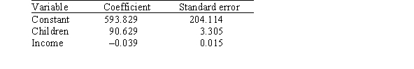
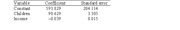
A researcher is investigating possible explanations for deaths in traffic accidents.He examined data from 1991 for each of the 50 states plus Washington,DC.The data included information on the following variables.  As part of his investigation he ran the multiple regression model, Deaths = 0 + 1(Children)+ 2(Income)+ i,
Where the deviations i were assumed to be independent and Normally distributed with a mean of 0 and a standard deviation of .This model was fit to the data using the method of least squares.The following results were obtained from statistical software.
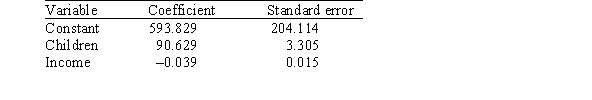 The researcher also ran the simple linear regression model
Deaths = 0 + 2(Income)+ i.
The following results were obtained from statistical software: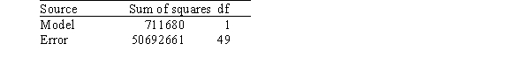
 What is the value of R2 in the simple linear regression model?
A)0.014
B)0.020
C)0.688
D)0.941
As part of his investigation he ran the multiple regression model, Deaths = 0 + 1(Children)+ 2(Income)+ i,Where the deviations i were assumed to be independent and Normally distributed with a mean of 0 and a standard deviation of .This model was fit to the data using the method of least squares.The following results were obtained from statistical software.
The researcher also ran the simple linear regression modelDeaths = 0 + 2(Income)+ i.
The following results were obtained from statistical software:
What is the value of R2 in the simple linear regression model?A)0.014
B)0.020
C)0.688
D)0.941
Question
A researcher is investigating possible explanations for deaths in traffic accidents.He examined data from 1991 for each of the 50 states plus Washington,DC.The data included information on the following variables.  As part of his investigation he ran the multiple regression model, Deaths = 0 + 1(Children)+ 2(Income)+ i,
Where the deviations i were assumed to be independent and Normally distributed with a mean of 0 and a standard deviation of .This model was fit to the data using the method of least squares.The following results were obtained from statistical software.
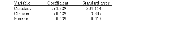 Suppose we wish to test the hypotheses H0: 1 = 2 = 0 versus Ha: at least one of the j is not 0 using the ANOVA F test.What can we say about the P-value for the ANOVA F test?
A)P-value < 0.001
B)0.001C)0.005 D)P-value > 0.01
As part of his investigation he ran the multiple regression model, Deaths = 0 + 1(Children)+ 2(Income)+ i,Where the deviations i were assumed to be independent and Normally distributed with a mean of 0 and a standard deviation of .This model was fit to the data using the method of least squares.The following results were obtained from statistical software.
Suppose we wish to test the hypotheses H0: 1 = 2 = 0 versus Ha: at least one of the j is not 0 using the ANOVA F test.What can we say about the P-value for the ANOVA F test?A)P-value < 0.001
B)0.001
Question
Based on a sample of the salaries of professors at a major university,you have performed a multiple linear regression relating salary to years of service and gender.The data included information on the following variables.  The estimated multiple linear regression model is Salary = 45 + 3(Years)+ 4(Gender)+ 1(Years)(Gender).
Using the multiple linear regression equation,what would you estimate the average difference in the salaries of a male professor with 3 years of service and a female professor with 3 years of service to be?
A)$3000
B)$4000
C)$5000
D)$7000
The estimated multiple linear regression model is Salary = 45 + 3(Years)+ 4(Gender)+ 1(Years)(Gender).Using the multiple linear regression equation,what would you estimate the average difference in the salaries of a male professor with 3 years of service and a female professor with 3 years of service to be?
A)$3000
B)$4000
C)$5000
D)$7000
Question
A researcher is investigating possible explanations for deaths in traffic accidents.He examined data from 1991 for each of the 50 states plus Washington,DC.The data included information on the following variables.  As part of his investigation he ran the multiple regression model, Deaths = 0 + 1(Children)+ 2(Income)+ i,
Where the deviations i were assumed to be independent and Normally distributed with a mean of 0 and a standard deviation of .This model was fit to the data using the method of least squares.The following results were obtained from statistical software.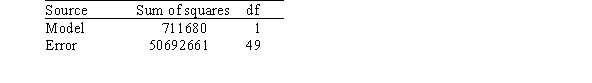
 The researcher also ran the simple linear regression model
Deaths = 0 + 2(Income)+ i.
The following results were obtained from statistical software:
 Based on the above results,the researcher tested the hypotheses H0: 2 = 0 versus Ha: 2 0.What do we know about the P-value of the test?
A)P-value < 0.025
B)0.025
C)0.05
D)P-value > 0.10
As part of his investigation he ran the multiple regression model, Deaths = 0 + 1(Children)+ 2(Income)+ i,Where the deviations i were assumed to be independent and Normally distributed with a mean of 0 and a standard deviation of .This model was fit to the data using the method of least squares.The following results were obtained from statistical software.
The researcher also ran the simple linear regression modelDeaths = 0 + 2(Income)+ i.
The following results were obtained from statistical software:
Based on the above results,the researcher tested the hypotheses H0: 2 = 0 versus Ha: 2 0.What do we know about the P-value of the test?A)P-value < 0.025
B)0.025
C)0.05
D)P-value > 0.10
Question
Question
Question
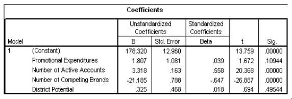
The data referred to in this question were collected from several sales districts across the country.The data represent sales for a maker of asphalt roofing shingles.Information on the following variables is available.  Partial SPSS regression output of a multiple regression model with sales as the response variable and the other four variables as predictor variables are given below.
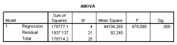
 What is a 95% confidence interval for the coefficient of promotional expenditures?
A)(-0.441,4.055)
B)(-0.312,3.926)
C)(-0.053,3.667)
D)(0.726,2.888)
Partial SPSS regression output of a multiple regression model with sales as the response variable and the other four variables as predictor variables are given below. What is a 95% confidence interval for the coefficient of promotional expenditures?A)(-0.441,4.055)
B)(-0.312,3.926)
C)(-0.053,3.667)
D)(0.726,2.888)
Question
The data referred to in this question were collected from several sales districts across the country.The data represent sales for a maker of asphalt roofing shingles.Information on the following variables is available.  Partial SPSS regression output of a multiple regression model with sales as the response variable and the other four variables as predictor variables are given below.
 What is the estimate for the error variance 2?
A)9.604
B)12.960
C)92.245
D)1937.137
Partial SPSS regression output of a multiple regression model with sales as the response variable and the other four variables as predictor variables are given below. What is the estimate for the error variance 2?A)9.604
B)12.960
C)92.245
D)1937.137
Question
The data referred to in this question were collected from several sales districts across the country.The data represent sales for a maker of asphalt roofing shingles.Information on the following variables is available.  Partial SPSS regression output of a multiple regression model with sales as the response variable and the other four variables as predictor variables are given below.
 In an attempt to increase sales,the company can only directly influence some of these variables.It cannot change the number of competitors;it cannot change the district potential.The only two variables they can actively change are the number of active accounts and the promotional expenditures.Suppose they have $5000 to spend on new commercials (that is,promotional expenditures).By how much are sales expected to increase?
A)1.807 squares
B)9.035 squares
C)1807 squares
D)9035 squares
Partial SPSS regression output of a multiple regression model with sales as the response variable and the other four variables as predictor variables are given below. In an attempt to increase sales,the company can only directly influence some of these variables.It cannot change the number of competitors;it cannot change the district potential.The only two variables they can actively change are the number of active accounts and the promotional expenditures.Suppose they have $5000 to spend on new commercials (that is,promotional expenditures).By how much are sales expected to increase?A)1.807 squares
B)9.035 squares
C)1807 squares
D)9035 squares
Question
A researcher is investigating possible explanations for deaths in traffic accidents.He examined data from 1991 for each of the 50 states plus Washington,DC.The data included information on the following variables.  As part of his investigation he ran the multiple regression model, Deaths = 0 + 1(Children)+ 2(Income)+ i,
Where the deviations i were assumed to be independent and Normally distributed with a mean of 0 and a standard deviation of .This model was fit to the data using the method of least squares.The following results were obtained from statistical software.
 The researcher also ran the simple linear regression model
Deaths = 0 + 2(Income)+ i.
The following results were obtained from statistical software: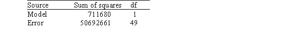
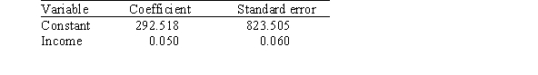 Based on the analyses,what can we conclude?
A)The variable income is statistically significant at level 0.05 as a predictor of the variable deaths.
B)The variable income is statistically significant at level 0.05 as a predictor of the variable deaths in a multiple regression model that includes the variable children.
C)The variable income is not useful as a predictor of the variable deaths and should be omitted from the analysis.
D)The variable children is not useful as a predictor of the variable deaths,unless the variable income is also present in the multiple regression model.
As part of his investigation he ran the multiple regression model, Deaths = 0 + 1(Children)+ 2(Income)+ i,Where the deviations i were assumed to be independent and Normally distributed with a mean of 0 and a standard deviation of .This model was fit to the data using the method of least squares.The following results were obtained from statistical software.
The researcher also ran the simple linear regression modelDeaths = 0 + 2(Income)+ i.
The following results were obtained from statistical software:
Based on the analyses,what can we conclude?A)The variable income is statistically significant at level 0.05 as a predictor of the variable deaths.
B)The variable income is statistically significant at level 0.05 as a predictor of the variable deaths in a multiple regression model that includes the variable children.
C)The variable income is not useful as a predictor of the variable deaths and should be omitted from the analysis.
D)The variable children is not useful as a predictor of the variable deaths,unless the variable income is also present in the multiple regression model.
Question
A researcher is investigating possible explanations for deaths in traffic accidents.He examined data from 1991 for each of the 50 states plus Washington,DC.The data included information on the following variables.  As part of his investigation he ran the multiple regression model, Deaths = 0 + 1(Children)+ 2(Income)+ i,
Where the deviations i were assumed to be independent and Normally distributed with a mean of 0 and a standard deviation of .This model was fit to the data using the method of least squares.The following results were obtained from statistical software.
 The researcher also ran the simple linear regression model
Deaths = 0 + 2(Income)+ i.
The following results were obtained from statistical software:
 What can we conclude regarding the meaningfulness of the analyses?
A)They are very meaningful because the results are based on a very large sample consisting of the people in all 50 states as well as Washington,DC.
B)They are meaningful because R2 for the multiple regression model is quite large,suggesting that the model fits well and the assumptions about the model are reasonable.
C)They are moderately meaningful because the results are based on a fairly large sample and they are at least consistent with what one would expect.They would be very meaningful if,in addition,we had examined the residuals and found no outliers or influential observations.
D)They are not necessarily meaningful because these results are based on available data.
As part of his investigation he ran the multiple regression model, Deaths = 0 + 1(Children)+ 2(Income)+ i,Where the deviations i were assumed to be independent and Normally distributed with a mean of 0 and a standard deviation of .This model was fit to the data using the method of least squares.The following results were obtained from statistical software.
The researcher also ran the simple linear regression modelDeaths = 0 + 2(Income)+ i.
The following results were obtained from statistical software:
What can we conclude regarding the meaningfulness of the analyses?A)They are very meaningful because the results are based on a very large sample consisting of the people in all 50 states as well as Washington,DC.
B)They are meaningful because R2 for the multiple regression model is quite large,suggesting that the model fits well and the assumptions about the model are reasonable.
C)They are moderately meaningful because the results are based on a fairly large sample and they are at least consistent with what one would expect.They would be very meaningful if,in addition,we had examined the residuals and found no outliers or influential observations.
D)They are not necessarily meaningful because these results are based on available data.
Question
Question
Question
Question
A researcher is investigating possible explanations for deaths in traffic accidents.He examined data from 1991 for each of the 50 states plus Washington,DC.The data included information on the following variables.  As part of his investigation he ran the multiple regression model, Deaths = 0 + 1(Children)+ 2(Income)+ i,
Where the deviations i were assumed to be independent and Normally distributed with a mean of 0 and a standard deviation of .This model was fit to the data using the method of least squares.The following results were obtained from statistical software.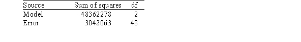
 Suppose we wish to test the hypotheses H0: 1 = 2 = 0 versus Ha: at least one of the j is not 0 using the ANOVA F test.What is the value of the F statistic?
A)0.94
B)15.9
C)24
D)381.5
As part of his investigation he ran the multiple regression model, Deaths = 0 + 1(Children)+ 2(Income)+ i,Where the deviations i were assumed to be independent and Normally distributed with a mean of 0 and a standard deviation of .This model was fit to the data using the method of least squares.The following results were obtained from statistical software.
Suppose we wish to test the hypotheses H0: 1 = 2 = 0 versus Ha: at least one of the j is not 0 using the ANOVA F test.What is the value of the F statistic?A)0.94
B)15.9
C)24
D)381.5
Question
The data referred to in this question were collected from several sales districts across the country.The data represent sales for a maker of asphalt roofing shingles.Information on the following variables is available.  Partial SPSS regression output of a multiple regression model with sales as the response variable and the other four variables as predictor variables are given below.
 What proportion of the variation in sales is explained by the set of all four explanatory variables?
A)-0.647
B)0.558
C)0.989
D)0.995
Partial SPSS regression output of a multiple regression model with sales as the response variable and the other four variables as predictor variables are given below. What proportion of the variation in sales is explained by the set of all four explanatory variables?A)-0.647
B)0.558
C)0.989
D)0.995
Question
The data referred to in this question were collected from several sales districts across the country.The data represent sales for a maker of asphalt roofing shingles.Information on the following variables is available.  Partial SPSS regression output of a multiple regression model with sales as the response variable and the other four variables as predictor variables are given below.
 Which of the four explanatory variables seems to be the least significant in the model?
A)Expenditures
B)Accounts
C)Competing brands
D)District potential
Partial SPSS regression output of a multiple regression model with sales as the response variable and the other four variables as predictor variables are given below. Which of the four explanatory variables seems to be the least significant in the model?A)Expenditures
B)Accounts
C)Competing brands
D)District potential
Question
A researcher is investigating possible explanations for deaths in traffic accidents.He examined data from 1991 for each of the 50 states plus Washington,DC.The data included information on the following variables.  As part of his investigation he ran the multiple regression model, Deaths = 0 + 1(Children)+ 2(Income)+ i,
Where the deviations i were assumed to be independent and Normally distributed with a mean of 0 and a standard deviation of .This model was fit to the data using the method of least squares.The following results were obtained from statistical software.
 What is a 99% confidence interval for 2,the coefficient of the variable income?
A)-0.039 ± 0.030
B)-0.039 ± 0.040
C)0.015 ± 0.079
D)0.015 ± 0.104
As part of his investigation he ran the multiple regression model, Deaths = 0 + 1(Children)+ 2(Income)+ i,Where the deviations i were assumed to be independent and Normally distributed with a mean of 0 and a standard deviation of .This model was fit to the data using the method of least squares.The following results were obtained from statistical software.
What is a 99% confidence interval for 2,the coefficient of the variable income?A)-0.039 ± 0.030
B)-0.039 ± 0.040
C)0.015 ± 0.079
D)0.015 ± 0.104
Question
The data referred to in this question were collected from several sales districts across the country.The data represent sales for a maker of asphalt roofing shingles.Information on the following variables is available.  Partial SPSS regression output of a multiple regression model with sales as the response variable and the other four variables as predictor variables are given below.
 An F test for the two coefficients of promotional expenditures and district potential is performed.The hypotheses are H0: 1 = 4 = 0 versus Ha: at least one of the j is not 0.The F statistic for this test is 1.482 with 2 and 21 degrees of freedom.What can we say about the P-value for this test?
A)P-value < 0.025
B)0.025
C)0.05
D)P-value > 0.10
Partial SPSS regression output of a multiple regression model with sales as the response variable and the other four variables as predictor variables are given below. An F test for the two coefficients of promotional expenditures and district potential is performed.The hypotheses are H0: 1 = 4 = 0 versus Ha: at least one of the j is not 0.The F statistic for this test is 1.482 with 2 and 21 degrees of freedom.What can we say about the P-value for this test?A)P-value < 0.025
B)0.025
C)0.05
D)P-value > 0.10
Question
The data referred to in this question were collected from several sales districts across the country.The data represent sales for a maker of asphalt roofing shingles.Information on the following variables is available.  Partial SPSS regression output of a multiple regression model with sales as the response variable and the other four variables as predictor variables are given below.
 How many districts were sampled in all?
A)21
B)24
C)25
D)26
Partial SPSS regression output of a multiple regression model with sales as the response variable and the other four variables as predictor variables are given below. How many districts were sampled in all?A)21
B)24
C)25
D)26
Question
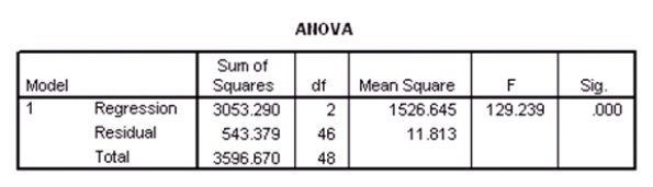
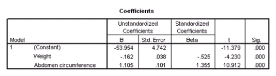
Researchers at a large nutrition and weight management company are trying to build a model to predict a person's body fat percentage from an array of variables such as body weight,height,and body measurements around the neck,chest,abdomen,hips,biceps,etc.A variable selection method is used to build a simple model.SPSS output for the final model is given below. 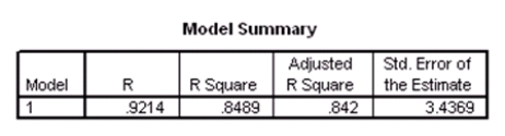
 A graph of the residuals versus the predicted values is given below.
 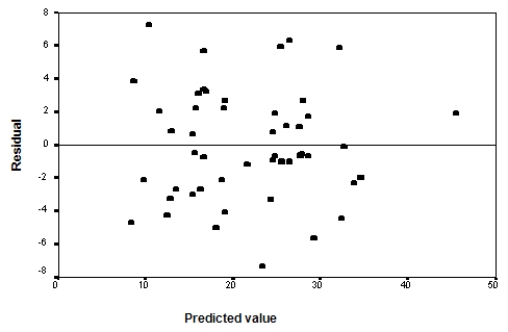 What assumption do we check with this graph?
A)The Normality of the error terms
B)The independence of the residuals
C)The constant variance assumption of the predicted values
D)None of the above
A graph of the residuals versus the predicted values is given below. What assumption do we check with this graph?A)The Normality of the error terms
B)The independence of the residuals
C)The constant variance assumption of the predicted values
D)None of the above
Question
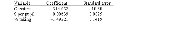
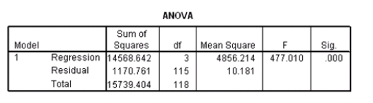
A researcher is investigating variables that might be associated with the academic performance of high school students.She examined data from 1990 for each of the 50 states plus Washington,DC.The data included information on the following variables.  As part of her investigation,she ran the multiple regression model SATM = 0 + 1($ per pupil)+ 2(% taking)+ i,
Where the deviations i were assumed to be independent and Normally distributed with a mean of 0 and a standard deviation of .This model was fit to the data using the method of least squares.The following results were obtained from statistical software.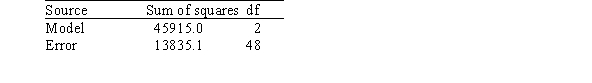
 Suppose we wish to test the hypotheses H0: 1 = 2 = 0 versus Ha: at least one of the j is not 0,using the ANOVA F test.What is the value of the F statistic?
A)3.32
B)24.0
C)79.65
D)159.3
As part of her investigation,she ran the multiple regression model SATM = 0 + 1($ per pupil)+ 2(% taking)+ i,Where the deviations i were assumed to be independent and Normally distributed with a mean of 0 and a standard deviation of .This model was fit to the data using the method of least squares.The following results were obtained from statistical software.
Suppose we wish to test the hypotheses H0: 1 = 2 = 0 versus Ha: at least one of the j is not 0,using the ANOVA F test.What is the value of the F statistic?A)3.32
B)24.0
C)79.65
D)159.3
Question
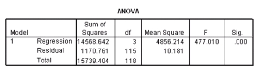
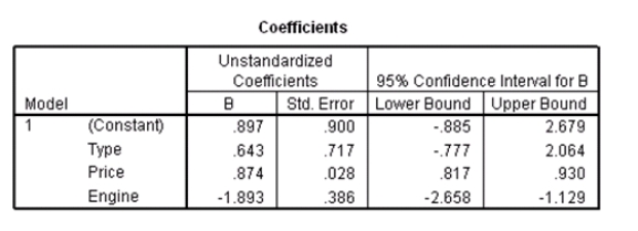
Researchers at a car resale company are trying to build a model to predict a car's 4-year resale value (in thousands of dollars)from several predictor variables.The variables they selected are as below.  Data were collected on cars of different models made by different manufacturers.SPSS output for the least-squares regression model is given below.
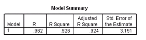

 A Normal quantile plot of the residuals is given below.
 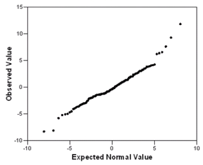 What assumption do we check with this graph,and does the assumption seem to be satisfied?
Data were collected on cars of different models made by different manufacturers.SPSS output for the least-squares regression model is given below. A Normal quantile plot of the residuals is given below. What assumption do we check with this graph,and does the assumption seem to be satisfied? Question
Based on a sample of the salaries of professors at a major university,you have performed a multiple linear regression relating salary to years of service and gender.The data included information on the following variables.  The estimated multiple linear regression model is Salary = 45 + 3(Years)+ 4(Gender)+ 1(Years)(Gender).
A particular female professor with 6 years of experience currently has a salary of $60,000.What is the residual for this observation?
A)-$9000
B)-$3000
C)$3000
D)$9000
The estimated multiple linear regression model is Salary = 45 + 3(Years)+ 4(Gender)+ 1(Years)(Gender).A particular female professor with 6 years of experience currently has a salary of $60,000.What is the residual for this observation?
A)-$9000
B)-$3000
C)$3000
D)$9000
Question
A researcher is investigating variables that might be associated with the academic performance of high school students.She examined data from 1990 for each of the 50 states plus Washington,DC.The data included information on the following variables.  As part of her investigation,she ran the multiple regression model SATM = 0 + 1($ per pupil)+ 2(% taking)+ i,
Where the deviations i were assumed to be independent and Normally distributed with a mean of 0 and a standard deviation of .This model was fit to the data using the method of least squares.The following results were obtained from statistical software.
 What proportion of the variation in the variable SATM is explained by the explanatory variables $ per pupil and % taking?
A)0.232
B)0.301
C)0.768
D)0.960
As part of her investigation,she ran the multiple regression model SATM = 0 + 1($ per pupil)+ 2(% taking)+ i,Where the deviations i were assumed to be independent and Normally distributed with a mean of 0 and a standard deviation of .This model was fit to the data using the method of least squares.The following results were obtained from statistical software.
What proportion of the variation in the variable SATM is explained by the explanatory variables $ per pupil and % taking?A)0.232
B)0.301
C)0.768
D)0.960
Question
A researcher is investigating variables that might be associated with the academic performance of high school students.She examined data from 1990 for each of the 50 states plus Washington,DC.The data included information on the following variables.  As part of her investigation,she ran the multiple regression model SATM = 0 + 1($ per pupil)+ 2(% taking)+ i,
Where the deviations i were assumed to be independent and Normally distributed with a mean of 0 and a standard deviation of .This model was fit to the data using the method of least squares.The following results were obtained from statistical software.
 Another researcher,using the same data,ran the simple linear regression model
SATM = 0 + 1($ per pupil)+ i.
The following results were obtained from statistical software.
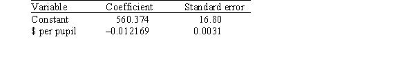 The first researcher concluded that because the coefficient for the variable $ per pupil was positive in her results,spending additional money on students would have a positive effect on SATM scores.This researcher therefore recommended more money be spent on students.The second researcher concluded that because the coefficient for the variable $ per pupil was negative in his results,spending additional money on students would have a negative effect on SATM scores.This researcher therefore recommended less money be spent on students.Why are these two conclusions different even though the researchers used the same data?
A)An error must have been made by one of the researchers.
B)Both researchers failed to take into account that in their analyses,1,the coefficient of the variable $ per pupil,was not statistically significant at even the 0.10 significance level.Hence,neither researcher could conclude that 1 was significantly different from zero.
C)The researchers did not use the same set of explanatory variables in their models.
D)There must have been an influential observation in the data,rendering the analyses inappropriate.
As part of her investigation,she ran the multiple regression model SATM = 0 + 1($ per pupil)+ 2(% taking)+ i,Where the deviations i were assumed to be independent and Normally distributed with a mean of 0 and a standard deviation of .This model was fit to the data using the method of least squares.The following results were obtained from statistical software.
Another researcher,using the same data,ran the simple linear regression modelSATM = 0 + 1($ per pupil)+ i.
The following results were obtained from statistical software.
The first researcher concluded that because the coefficient for the variable $ per pupil was positive in her results,spending additional money on students would have a positive effect on SATM scores.This researcher therefore recommended more money be spent on students.The second researcher concluded that because the coefficient for the variable $ per pupil was negative in his results,spending additional money on students would have a negative effect on SATM scores.This researcher therefore recommended less money be spent on students.Why are these two conclusions different even though the researchers used the same data?A)An error must have been made by one of the researchers.
B)Both researchers failed to take into account that in their analyses,1,the coefficient of the variable $ per pupil,was not statistically significant at even the 0.10 significance level.Hence,neither researcher could conclude that 1 was significantly different from zero.
C)The researchers did not use the same set of explanatory variables in their models.
D)There must have been an influential observation in the data,rendering the analyses inappropriate.
Question
Researchers at a car resale company are trying to build a model to predict a car's 4-year resale value (in thousands of dollars)from several predictor variables.The variables they selected are as below.  Data were collected on cars of different models made by different manufacturers.SPSS output for the least-squares regression model is given below.
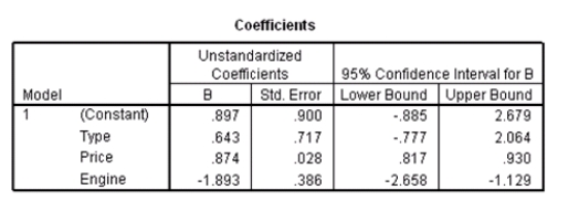 A particular car (not a truck)cost $40,000 and has an engine of 3.8 liters.What do you predict the 4-year resale value of this car to be?
Data were collected on cars of different models made by different manufacturers.SPSS output for the least-squares regression model is given below. A particular car (not a truck)cost $40,000 and has an engine of 3.8 liters.What do you predict the 4-year resale value of this car to be? Question
Researchers at a large nutrition and weight management company are trying to build a model to predict a person's body fat percentage from an array of variables such as body weight,height,and body measurements around the neck,chest,abdomen,hips,biceps,etc.A variable selection method is used to build a simple model.SPSS output for the final model is given below. 

 What percentage of the variation in percent body fat remains unexplained,even after introducing weight and abdomen circumference into the model?
A)7.86%
B)15.11%
C)84.89%
D)92.14%
What percentage of the variation in percent body fat remains unexplained,even after introducing weight and abdomen circumference into the model?A)7.86%
B)15.11%
C)84.89%
D)92.14%
Question
Researchers at a car resale company are trying to build a model to predict a car's 4-year resale value (in thousands of dollars)from several predictor variables.The variables they selected are as below.  Data were collected on cars of different models made by different manufacturers.SPSS output for the least-squares regression model is given below.
 Suppose we wish to test the hypotheses H0: 1 = 0 versus Ha: 1 0,where 1 is the coefficient for the variable type.Based on the 95% confidence interval given in the output,what do we know about the value of the P-value of this test?
Data were collected on cars of different models made by different manufacturers.SPSS output for the least-squares regression model is given below. Suppose we wish to test the hypotheses H0: 1 = 0 versus Ha: 1 0,where 1 is the coefficient for the variable type.Based on the 95% confidence interval given in the output,what do we know about the value of the P-value of this test? Question
Based on a sample of the salaries of professors at a major university,you have performed a multiple linear regression relating salary to years of service and gender.The data included information on the following variables.  The estimated multiple linear regression model is Salary = 45 + 3(Years)+ 4(Gender)+ 1(Years)(Gender).
Using the multiple linear regression equation,what would you estimate the average salary of male professors with 3 years of experience to be?
A)$53,000
B)$54,000
C)$58,000
D)$61,000
The estimated multiple linear regression model is Salary = 45 + 3(Years)+ 4(Gender)+ 1(Years)(Gender).Using the multiple linear regression equation,what would you estimate the average salary of male professors with 3 years of experience to be?
A)$53,000
B)$54,000
C)$58,000
D)$61,000
Question
A researcher is investigating variables that might be associated with the academic performance of high school students.She examined data from 1990 for each of the 50 states plus Washington,DC.The data included information on the following variables.  As part of her investigation,she ran the multiple regression model SATM = 0 + 1($ per pupil)+ 2(% taking)+ i,
Where the deviations i were assumed to be independent and Normally distributed with a mean of 0 and a standard deviation of .This model was fit to the data using the method of least squares.The following results were obtained from statistical software.
 What is the value of the MSE?
A)10.30
B)288.23
C)13835.10
D)22957.50
As part of her investigation,she ran the multiple regression model SATM = 0 + 1($ per pupil)+ 2(% taking)+ i,Where the deviations i were assumed to be independent and Normally distributed with a mean of 0 and a standard deviation of .This model was fit to the data using the method of least squares.The following results were obtained from statistical software.
What is the value of the MSE?A)10.30
B)288.23
C)13835.10
D)22957.50
Question
Researchers at a large nutrition and weight management company are trying to build a model to predict a person's body fat percentage from an array of variables such as body weight,height,and body measurements around the neck,chest,abdomen,hips,biceps,etc.A variable selection method is used to build a simple model.SPSS output for the final model is given below. 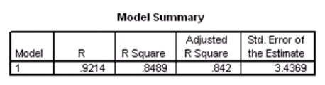

 How many people were included in the study?
A)46
B)48
C)49
D)50
How many people were included in the study?A)46
B)48
C)49
D)50
Question
A researcher is investigating variables that might be associated with the academic performance of high school students.She examined data from 1990 for each of the 50 states plus Washington,DC.The data included information on the following variables.  As part of her investigation,she ran the multiple regression model SATM = 0 + 1($ per pupil)+ 2(% taking)+ i,
Where the deviations i were assumed to be independent and Normally distributed with a mean of 0 and a standard deviation of .This model was fit to the data using the method of least squares.The following results were obtained from statistical software.
 What is an approximate 95% confidence interval for 1,the coefficient of the variable $ per pupil?
A)0.00639 ± 0.0025
B)0.00639 ± 0.0042
C)0.00639 ± 0.0050
D)0.00639 ± 0.0067
As part of her investigation,she ran the multiple regression model SATM = 0 + 1($ per pupil)+ 2(% taking)+ i,Where the deviations i were assumed to be independent and Normally distributed with a mean of 0 and a standard deviation of .This model was fit to the data using the method of least squares.The following results were obtained from statistical software.
What is an approximate 95% confidence interval for 1,the coefficient of the variable $ per pupil?A)0.00639 ± 0.0025
B)0.00639 ± 0.0042
C)0.00639 ± 0.0050
D)0.00639 ± 0.0067
Question
A researcher is investigating variables that might be associated with the academic performance of high school students.She examined data from 1990 for each of the 50 states plus Washington,DC.The data included information on the following variables.  As part of her investigation,she ran the multiple regression model SATM = 0 + 1($ per pupil)+ 2(% taking)+ i,
Where the deviations i were assumed to be independent and Normally distributed with a mean of 0 and a standard deviation of .This model was fit to the data using the method of least squares.The following results were obtained from statistical software.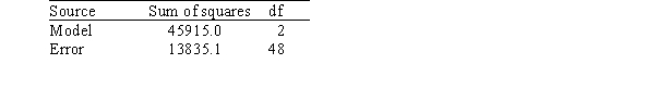
 Another researcher,using the same data,ran the simple linear regression model
SATM = 0 + 1($ per pupil)+ i.
The following results were obtained from statistical software.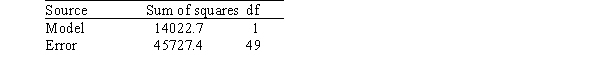
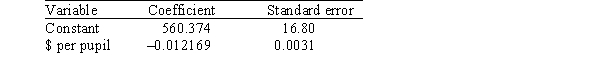 Based on these results,a 95% confidence interval for 1,the coefficient of the variable $ per pupil,is approximately
A)-0.012169 ± 0.0031.
B)-0.012169 ± 0.0052.
C)-0.012169 ± 0.0062.
D)-0.012169 ± 0.0083.
As part of her investigation,she ran the multiple regression model SATM = 0 + 1($ per pupil)+ 2(% taking)+ i,Where the deviations i were assumed to be independent and Normally distributed with a mean of 0 and a standard deviation of .This model was fit to the data using the method of least squares.The following results were obtained from statistical software.
Another researcher,using the same data,ran the simple linear regression modelSATM = 0 + 1($ per pupil)+ i.
The following results were obtained from statistical software.
Based on these results,a 95% confidence interval for 1,the coefficient of the variable $ per pupil,is approximatelyA)-0.012169 ± 0.0031.
B)-0.012169 ± 0.0052.
C)-0.012169 ± 0.0062.
D)-0.012169 ± 0.0083.
Question
Researchers at a large nutrition and weight management company are trying to build a model to predict a person's body fat percentage from an array of variables such as body weight,height,and body measurements around the neck,chest,abdomen,hips,biceps,etc.A variable selection method is used to build a simple model.SPSS output for the final model is given below. 

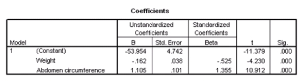 What is a 90% confidence interval for 1,the coefficient of weight,based on these results?
A)-0.162 ± 0.038
B)-0.162 ± 0.064
C)-0.162 ± 0.525
D)-0.162 ± 4.230
What is a 90% confidence interval for 1,the coefficient of weight,based on these results?A)-0.162 ± 0.038
B)-0.162 ± 0.064
C)-0.162 ± 0.525
D)-0.162 ± 4.230
Question
Researchers at a car resale company are trying to build a model to predict a car's 4-year resale value (in thousands of dollars)from several predictor variables.The variables they selected are as below.  Data were collected on cars of different models made by different manufacturers.SPSS output for the least-squares regression model is given below.

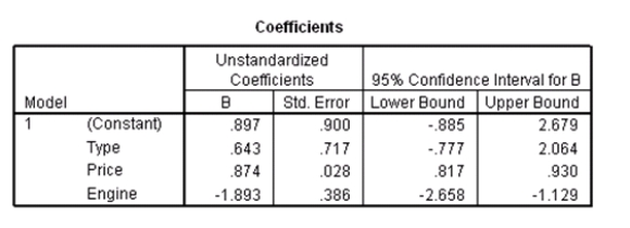 An F test for the two coefficients of type and engine is performed.The hypotheses areH0: 1 = 3 = 0 versus Ha: at least one of the j is not 0.The F statistic for this test is 12.21 with 2 and 115 degrees of freedom.Do we reject the null hypothesis at the 5% significance level?
Data were collected on cars of different models made by different manufacturers.SPSS output for the least-squares regression model is given below. An F test for the two coefficients of type and engine is performed.The hypotheses areH0: 1 = 3 = 0 versus Ha: at least one of the j is not 0.The F statistic for this test is 12.21 with 2 and 115 degrees of freedom.Do we reject the null hypothesis at the 5% significance level? Question
Researchers at a car resale company are trying to build a model to predict a car's 4-year resale value (in thousands of dollars)from several predictor variables.The variables they selected are as below.  Data were collected on cars of different models made by different manufacturers.SPSS output for the least-squares regression model is given below.
 What is the equation of the least-squares regression line?
Data were collected on cars of different models made by different manufacturers.SPSS output for the least-squares regression model is given below. What is the equation of the least-squares regression line? Question
Researchers at a large nutrition and weight management company are trying to build a model to predict a person's body fat percentage from an array of variables such as body weight,height,and body measurements around the neck,chest,abdomen,hips,biceps,etc.A variable selection method is used to build a simple model.SPSS output for the final model is given below. 
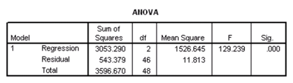
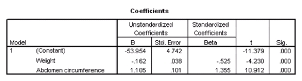 What is the value of an estimate of 2?
A)3.4369
B)11.813
C)543.379
D)1526.645
What is the value of an estimate of 2?A)3.4369
B)11.813
C)543.379
D)1526.645
Question
Researchers at a large nutrition and weight management company are trying to build a model to predict a person's body fat percentage from an array of variables such as body weight,height,and body measurements around the neck,chest,abdomen,hips,biceps,etc.A variable selection method is used to build a simple model.SPSS output for the final model is given below. 

 Suppose we wish to test the hypotheses H0: 1 = 2 = 0 versus Ha: at least one of the j is not 0,using the ANOVA F test.What is the value of the test statistic?
A)-11.379
B)-4.230
C)10.912
D)129.239
Suppose we wish to test the hypotheses H0: 1 = 2 = 0 versus Ha: at least one of the j is not 0,using the ANOVA F test.What is the value of the test statistic?A)-11.379
B)-4.230
C)10.912
D)129.239
Question
Researchers at a car resale company are trying to build a model to predict a car's 4-year resale value (in thousands of dollars)from several predictor variables.The variables they selected are as below.  Data were collected on cars of different models made by different manufacturers.SPSS output for the least-squares regression model is given below.

 What is the value of an estimate for the error standard deviation ?
Data were collected on cars of different models made by different manufacturers.SPSS output for the least-squares regression model is given below. What is the value of an estimate for the error standard deviation ? Question
The NFL keeps track of a large number of statistics during the football season.For 2009 the number of points scored per game and how it related to such variables as the number of passes attempted per game (PassAtt/G),the total pass yards gained during the season (PassYds),and the total rushing yards gained in the season (RushYds)were studied.The following tables provide information on the least-squares fit of a multiple regression model for Pts/G on the three explanatory variables. 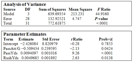 What would be the 96% confidence interval estimate for the true regression coefficient for the variable PassAtt/G?
A)(-0.080,0.001)
B)(-1.025,0.007)
C)(-0.007,1.025)
D)(-5.203,4.185)
E)Not within ± 0.02 of any of the above
What would be the 96% confidence interval estimate for the true regression coefficient for the variable PassAtt/G?A)(-0.080,0.001)
B)(-1.025,0.007)
C)(-0.007,1.025)
D)(-5.203,4.185)
E)Not within ± 0.02 of any of the above
Question
In this experiment,the risk-taking propensity of 90 inner city drug users was measured using a repeated measures test called the Behavioral Analogue Risk Task (BART;Lejuez et al. ,2002).The higher the BART score,the higher the risk-taking propensity.Participants also filled out questionnaires so that their Psychopathic Personality Inventory (PPI)scores could be computed.PPI scores are used to detect psychopathic traits in a covert manner and are a common indicator of one's level of psychopathy.The main goal of the experiment was to examine the relationship between risk-taking (measured by BART)based on one's level of psychopathy (measured by PPI on a scale of 0-100),gender (1 for male and 2 for female),and heroin use (1 for heroin use and 0 for no heroin use).Below is a partial output of a multiple regression analysis.  What are the explanatory variables in this study?
A)Gender and Bart score
B)Gender and PPI
C)Gender,heroin,and PPI
What are the explanatory variables in this study?A)Gender and Bart score
B)Gender and PPI
C)Gender,heroin,and PPI
Question
A study was conducted on 40 different brands of golf balls with respect to the distance the ball traveled after being struck with standardized test 7-iron.The response variable DIST is the measurement of the carry distance of the shot in yards.The explanatory variables are SMASH,the ratio of the ball speed/club speed at impact;SPIN,the initial spin rate of the ball in RPMs;and HEIGHT,the peak height of the ball in flight measured in feet. The following is a table showing some computer output (missing results are shown by **)for a least-squares fit of a multiple regression model using these variables. 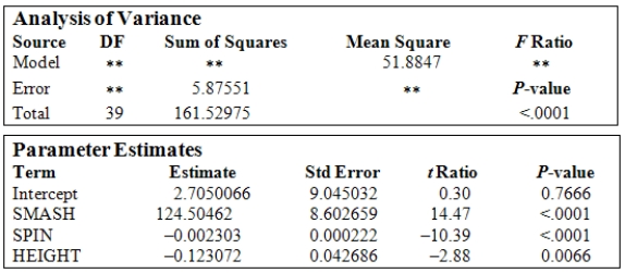 What is the value of the squared multiple correlation
  ?
?
A)0.036
B)0.960
C)0.163
D)0.964
E)0.404
What is the value of the squared multiple correlation ?A)0.036
B)0.960
C)0.163
D)0.964
E)0.404
Question
A study was conducted on 40 different brands of golf balls with respect to the distance the ball traveled after being struck with standardized test 7-iron.The response variable DIST is the measurement of the carry distance of the shot in yards.The explanatory variables are SMASH,the ratio of the ball speed/club speed at impact;SPIN,the initial spin rate of the ball in RPMs;and HEIGHT,the peak height of the ball in flight measured in feet. The following is a table showing some computer output (missing results are shown by **)for a least-squares fit of a multiple regression model using these variables.  Based upon the P-value of the ANOVA F test,what can be concluded about the relationship between the response variable and the explanatory variables?
A)A significant amount of the variation in the response variable can be explained by the regression on the explanatory variables.
B)There is strong evidence that the distance a golf ball travels depends upon the variable SMASH.
C)There is strong statistical evidence that at least one of the regression coefficients is not equal to zero.
D)When considered on its own,the variable SPIN is significantly different from zero.
E)There is strong statistical evidence that none of the regression coefficients is equal and all are significantly different from zero.
Based upon the P-value of the ANOVA F test,what can be concluded about the relationship between the response variable and the explanatory variables?A)A significant amount of the variation in the response variable can be explained by the regression on the explanatory variables.
B)There is strong evidence that the distance a golf ball travels depends upon the variable SMASH.
C)There is strong statistical evidence that at least one of the regression coefficients is not equal to zero.
D)When considered on its own,the variable SPIN is significantly different from zero.
E)There is strong statistical evidence that none of the regression coefficients is equal and all are significantly different from zero.
Question
In this experiment,the risk-taking propensity of 90 inner city drug users was measured using a repeated measures test called the Behavioral Analogue Risk Task (BART;Lejuez et al. ,2002).The higher the BART score,the higher the risk-taking propensity.Participants also filled out questionnaires so that their Psychopathic Personality Inventory (PPI)scores could be computed.PPI scores are used to detect psychopathic traits in a covert manner and are a common indicator of one's level of psychopathy.The main goal of the experiment was to examine the relationship between risk-taking (measured by BART)based on one's level of psychopathy (measured by PPI on a scale of 0-100),gender (1 for male and 2 for female),and heroin use (1 for heroin use and 0 for no heroin use).Below is a partial output of a multiple regression analysis.  What proportion of the variation of the response variable is explained by the explanatory variables?
A)4.48%
B)20%
C)2%
D)40%
What proportion of the variation of the response variable is explained by the explanatory variables?A)4.48%
B)20%
C)2%
D)40%
Question
In this experiment,the risk-taking propensity of 90 inner city drug users was measured using a repeated measures test called the Behavioral Analogue Risk Task (BART;Lejuez et al. ,2002).The higher the BART score,the higher the risk-taking propensity.Participants also filled out questionnaires so that their Psychopathic Personality Inventory (PPI)scores could be computed.PPI scores are used to detect psychopathic traits in a covert manner and are a common indicator of one's level of psychopathy.The main goal of the experiment was to examine the relationship between risk-taking (measured by BART)based on one's level of psychopathy (measured by PPI on a scale of 0-100),gender (1 for male and 2 for female),and heroin use (1 for heroin use and 0 for no heroin use).Below is a partial output of a multiple regression analysis.  Based on this model,are heroin users bigger risktakers than non-heroin users?
A)Yes
B)No
Based on this model,are heroin users bigger risktakers than non-heroin users?A)Yes
B)No
Question
Data were obtained in a study of the oxygen uptake of 31 middle-aged-males and females while exercising.The researchers were interested in the use of a variety of variables as predictors of Oxygen Uptake.The variables that were measured on the subjects were Age,Weight,the time taken to run a specified distance (Runtime),pulse rate at the end of the run (RunPulse),their resting pulse rate (RstPulse),and their maximum pulse rate during the run (MaxPulse).The following table from a computer analysis of the data is provided (with some entries deleted and replaced by **).  What is the mean square for model (MSM)?
A)144.293
B)120.244
C)721.463
D)180.366
E)141.897
What is the mean square for model (MSM)?A)144.293
B)120.244
C)721.463
D)180.366
E)141.897
Question
In this experiment,the risk-taking propensity of 90 inner city drug users was measured using a repeated measures test called the Behavioral Analogue Risk Task (BART;Lejuez et al. ,2002).The higher the BART score,the higher the risk-taking propensity.Participants also filled out questionnaires so that their Psychopathic Personality Inventory (PPI)scores could be computed.PPI scores are used to detect psychopathic traits in a covert manner and are a common indicator of one's level of psychopathy.The main goal of the experiment was to examine the relationship between risk-taking (measured by BART)based on one's level of psychopathy (measured by PPI on a scale of 0-100),gender (1 for male and 2 for female),and heroin use (1 for heroin use and 0 for no heroin use).Below is a partial output of a multiple regression analysis.  Does this model seem like an adequate model to predict risk-taking propensity?
A)No,the R-squared value is very low and most of the variables are not statistically significant.
B)Yes,the r correlation is very strong.
C)This cannot be determined from the given information.
Does this model seem like an adequate model to predict risk-taking propensity?A)No,the R-squared value is very low and most of the variables are not statistically significant.
B)Yes,the r correlation is very strong.
C)This cannot be determined from the given information.
Question
The NFL keeps track of a large number of statistics during the football season.For 2009 the number of points scored per game and how it related to such variables as the number of passes attempted per game (PassAtt/G),the total pass yards gained during the season (PassYds),and the total rushing yards gained in the season (RushYds)were studied.The following tables provide information on the least-squares fit of a multiple regression model for Pts/G on the three explanatory variables.  If a team were to attempt 30 passes per game,pass for a total of 3500 yards,and rush for 2000 yards,what would the fitted regression model predict for the points the team would score per game?
A)25.2
B)27.6
C)44.9
D)58.2
E)18.8
If a team were to attempt 30 passes per game,pass for a total of 3500 yards,and rush for 2000 yards,what would the fitted regression model predict for the points the team would score per game?A)25.2
B)27.6
C)44.9
D)58.2
E)18.8
Question
Data were obtained in a study of the oxygen uptake of 31 middle-aged-males and females while exercising.The researchers were interested in the use of a variety of variables as predictors of Oxygen Uptake.The variables that were measured on the subjects were Age,Weight,the time taken to run a specified distance (Runtime),pulse rate at the end of the run (RunPulse),their resting pulse rate (RstPulse),and their maximum pulse rate during the run (MaxPulse).The following table from a computer analysis of the data is provided (with some entries deleted and replaced by **).  What is the value of the F statistic and the associated degrees of freedom for the test?
A)F = 5.55 and DF = 6,30
B)F = 5.55 and DF = 6,24
C)F = 22.21 and DF = 6,30
D)F = 22.21 and DF = 5,24
E)F = 22.21 and DF = 6,24
What is the value of the F statistic and the associated degrees of freedom for the test?A)F = 5.55 and DF = 6,30
B)F = 5.55 and DF = 6,24
C)F = 22.21 and DF = 6,30
D)F = 22.21 and DF = 5,24
E)F = 22.21 and DF = 6,24
Question
Which of the following statements about the statistical model for multiple linear regression, 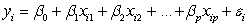 ,i = 1,2,…,n,is/are FALSE?
A)The deviations are independent.
B)The mean response is a linear function of the explanatory variables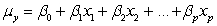 .
.
C)The parameters of the model are ,p,and .
D)The deviations are Normally distributed with a mean of 0 and a standard deviation of .
E)The deviations are a simple random sample from the N(0,)distribution.
,i = 1,2,…,n,is/are FALSE?A)The deviations
are independent.B)The mean response is a linear function of the explanatory variables
.C)The parameters of the model are
,p,and .D)The deviations
are Normally distributed with a mean of 0 and a standard deviation of .E)The deviations
are a simple random sample from the N(0,)distribution. Question
Data were obtained in a study of the oxygen uptake of 31 middle-aged-males and females while exercising.The researchers were interested in the use of a variety of variables as predictors of Oxygen Uptake.The variables that were measured on the subjects were Age,Weight,the time taken to run a specified distance (Runtime),pulse rate at the end of the run (RunPulse),their resting pulse rate (RstPulse),and their maximum pulse rate during the run (MaxPulse).The following table from a computer analysis of the data is provided (with some entries deleted and replaced by **). 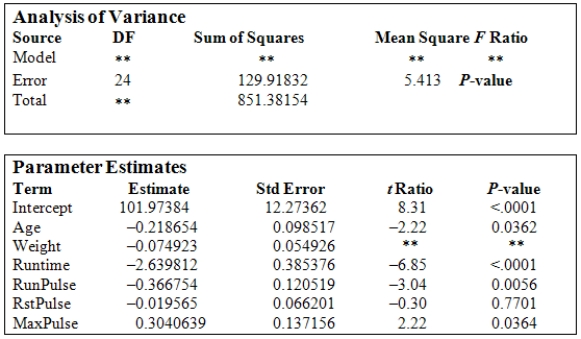 Under H0:
  against Ha:
  to test the significance of the variable Weight,what are the values of the test statistic and the P-value of the test?
A)t = 1.36 and the P-value is between 0.1 and 0.2.
B)t = -1.36 and the P-value is between 0.05 and 0.1.
C)t = -1.36 and the P-value is between 0.1 and 0.2.
D)t = -1.36 and the P-value is greater than 0.2.
E)t = 1.36;and the P-value is between 0.05 and 0.1.
Under H0: against Ha: to test the significance of the variable Weight,what are the values of the test statistic and the P-value of the test?A)t = 1.36 and the P-value is between 0.1 and 0.2.
B)t = -1.36 and the P-value is between 0.05 and 0.1.
C)t = -1.36 and the P-value is between 0.1 and 0.2.
D)t = -1.36 and the P-value is greater than 0.2.
E)t = 1.36;and the P-value is between 0.05 and 0.1.
Question
In this experiment,the risk-taking propensity of 90 inner city drug users was measured using a repeated measures test called the Behavioral Analogue Risk Task (BART;Lejuez et al. ,2002).The higher the BART score,the higher the risk-taking propensity.Participants also filled out questionnaires so that their Psychopathic Personality Inventory (PPI)scores could be computed.PPI scores are used to detect psychopathic traits in a covert manner and are a common indicator of one's level of psychopathy.The main goal of the experiment was to examine the relationship between risk-taking (measured by BART)based on one's level of psychopathy (measured by PPI on a scale of 0-100),gender (1 for male and 2 for female),and heroin use (1 for heroin use and 0 for no heroin use).Below is a partial output of a multiple regression analysis.  What is the response variable in this study?
A)Gender and Bart score
B)BART score
C)Gender and PPI
D)Gender,heroin,and PPI
What is the response variable in this study?A)Gender and Bart score
B)BART score
C)Gender and PPI
D)Gender,heroin,and PPI
Question
Data were obtained in a study of the oxygen uptake of 31 middle-aged-males and females while exercising.The researchers were interested in the use of a variety of variables as predictors of Oxygen Uptake.The variables that were measured on the subjects were Age,Weight,the time taken to run a specified distance (Runtime),pulse rate at the end of the run (RunPulse),their resting pulse rate (RstPulse),and their maximum pulse rate during the run (MaxPulse).The following table from a computer analysis of the data is provided (with some entries deleted and replaced by **).  What would the appropriate hypotheses be for testing the regression coefficients using the F ratio in the above table?
A)H0:
Ha:
B)H0:
Ha: at least one of the
 is not 0
C)H0:
Ha:
D)H0: all the = 0
= 0
Ha: all the
 0
0
E)H0: at most all of the = 0
= 0
Ha: at least one or more of the
 = 0
= 0
What would the appropriate hypotheses be for testing the regression coefficients using the F ratio in the above table?A)H0:
Ha:
B)H0:
Ha: at least one of the
is not 0C)H0:
Ha:
D)H0: all the
= 0Ha: all the
0E)H0: at most all of the
= 0Ha: at least one or more of the
= 0 Question
Data were obtained in a study of the oxygen uptake of 31 middle-aged-males and females while exercising.The researchers were interested in the use of a variety of variables as predictors of Oxygen Uptake.The variables that were measured on the subjects were Age,Weight,the time taken to run a specified distance (Runtime),pulse rate at the end of the run (RunPulse),their resting pulse rate (RstPulse),and their maximum pulse rate during the run (MaxPulse).The following table from a computer analysis of the data is provided (with some entries deleted and replaced by **).  In the above computer output we note that the t ratio for the variable RunPulse is -3.04,with a P-value of 0.0056.What is the best interpretation of this result?
A)The small P-value suggests that the variable RunPulse is not a significant predictor of Oxygen Uptake.
B)There is strong evidence that RunPulse is an important variable.
C)When assessing the value of variables for predicting Oxygen Uptake,the variable RunPulse by itself is very important.
D)The small P-value suggests that the variable RunPulse is statistically significant when all the other predictor variables are included in the regression equation.
E)The regression equation should include RunPulse since it is a statistically significant variable.
In the above computer output we note that the t ratio for the variable RunPulse is -3.04,with a P-value of 0.0056.What is the best interpretation of this result?A)The small P-value suggests that the variable RunPulse is not a significant predictor of Oxygen Uptake.
B)There is strong evidence that RunPulse is an important variable.
C)When assessing the value of variables for predicting Oxygen Uptake,the variable RunPulse by itself is very important.
D)The small P-value suggests that the variable RunPulse is statistically significant when all the other predictor variables are included in the regression equation.
E)The regression equation should include RunPulse since it is a statistically significant variable.
Question
In this experiment,the risk-taking propensity of 90 inner city drug users was measured using a repeated measures test called the Behavioral Analogue Risk Task (BART;Lejuez et al. ,2002).The higher the BART score,the higher the risk-taking propensity.Participants also filled out questionnaires so that their Psychopathic Personality Inventory (PPI)scores could be computed.PPI scores are used to detect psychopathic traits in a covert manner and are a common indicator of one's level of psychopathy.The main goal of the experiment was to examine the relationship between risk-taking (measured by BART)based on one's level of psychopathy (measured by PPI on a scale of 0-100),gender (1 for male and 2 for female),and heroin use (1 for heroin use and 0 for no heroin use).Below is a partial output of a multiple regression analysis.  Based on this model,are men bigger risktakers than women?
A)Yes
B)No
Based on this model,are men bigger risktakers than women?A)Yes
B)No
Question
In this experiment,the risk-taking propensity of 90 inner city drug users was measured using a repeated measures test called the Behavioral Analogue Risk Task (BART;Lejuez et al. ,2002).The higher the BART score,the higher the risk-taking propensity.Participants also filled out questionnaires so that their Psychopathic Personality Inventory (PPI)scores could be computed.PPI scores are used to detect psychopathic traits in a covert manner and are a common indicator of one's level of psychopathy.The main goal of the experiment was to examine the relationship between risk-taking (measured by BART)based on one's level of psychopathy (measured by PPI on a scale of 0-100),gender (1 for male and 2 for female),and heroin use (1 for heroin use and 0 for no heroin use).Below is a partial output of a multiple regression analysis.  How many explanatory variables are in this study?
A)One
B)Two
C)Three
How many explanatory variables are in this study?A)One
B)Two
C)Three
Question
A study was conducted on 40 different brands of golf balls with respect to the distance the ball traveled after being struck with standardized test 7-iron.The response variable DIST is the measurement of the carry distance of the shot in yards.The explanatory variables are SMASH,the ratio of the ball speed/club speed at impact;SPIN,the initial spin rate of the ball in RPMs;and HEIGHT,the peak height of the ball in flight measured in feet. The following is a table showing some computer output (missing results are shown by **)for a least-squares fit of a multiple regression model using these variables.  What is the estimate of the parameter
  ?
?
A)0.404
B)0.163
C)51.885
D)7.203
E)4.141
What is the estimate of the parameter ?A)0.404
B)0.163
C)51.885
D)7.203
E)4.141
Question
Data were obtained in a study of the oxygen uptake of 31 middle-aged-males and females while exercising.The researchers were interested in the use of a variety of variables as predictors of Oxygen Uptake.The variables that were measured on the subjects were Age,Weight,the time taken to run a specified distance (Runtime),pulse rate at the end of the run (RunPulse),their resting pulse rate (RstPulse),and their maximum pulse rate during the run (MaxPulse).The following table from a computer analysis of the data is provided (with some entries deleted and replaced by **). 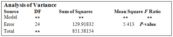 The degrees of freedom for model (DFM)and total (DFT)are
A)DFM = 5 and DFT = 31.
B)DFM = 4 and DFT = 30.
C)DFM = 6 and DFT = 31.
D)DFM = 6 and DFT = 30.
E)DFM = 5 and DFT = 30.
The degrees of freedom for model (DFM)and total (DFT)areA)DFM = 5 and DFT = 31.
B)DFM = 4 and DFT = 30.
C)DFM = 6 and DFT = 31.
D)DFM = 6 and DFT = 30.
E)DFM = 5 and DFT = 30.
Question
Question
Question
Question
Campus crime rates are generally lower than the national average;however thousands of crimes take place on college campuses daily.Cities that are notoriously dangerous would likely be undesirable locations for a college campus.A study examined the crime rates on campuses throughout the United States and whether or not they were significantly affected by surrounding cities.A regression analysis was performed to investigate which characteristics of a city,along with a few chosen demographics of a school,impacted the crime rate on a college campus.There are over 4000 colleges and universities in the United States.The study included a random sample of 129 institutions.The response variable was the number of crimes per 1000 people.Explanatory variables included the percent of married couples in the city (married),tuition of the university (tuition),average income of the city (income),unemployment rate of the city (unemployment),percent of students who belong to a fraternity or sorority (Greek),average age of the students at the university (age),and number of liquor stores in the city (liquor).A complete analysis of the data is shown below. 


 Examine the Q-Q plot of the residuals.What do you notice?
A)The Q-Q plot indicates some deviations from Normality,which could invalidate the analyses.
B)The residuals appear Normal;therefore,the regression results are accurate.
C)The residuals should be checked using a boxplot instead of a Q-Q plot.Not enough information can be obtained from the Q-Q plot.
D)One cannot obtain any information about the model from the residuals.
Examine the Q-Q plot of the residuals.What do you notice?A)The Q-Q plot indicates some deviations from Normality,which could invalidate the analyses.
B)The residuals appear Normal;therefore,the regression results are accurate.
C)The residuals should be checked using a boxplot instead of a Q-Q plot.Not enough information can be obtained from the Q-Q plot.
D)One cannot obtain any information about the model from the residuals.
Question
Question
Campus crime rates are generally lower than the national average;however thousands of crimes take place on college campuses daily.Cities that are notoriously dangerous would likely be undesirable locations for a college campus.A study examined the crime rates on campuses throughout the United States and whether or not they were significantly affected by surrounding cities.A regression analysis was performed to investigate which characteristics of a city,along with a few chosen demographics of a school,impacted the crime rate on a college campus.There are over 4000 colleges and universities in the United States.The study included a random sample of 129 institutions.The response variable was the number of crimes per 1000 people.Explanatory variables included the percent of married couples in the city (married),tuition of the university (tuition),average income of the city (income),unemployment rate of the city (unemployment),percent of students who belong to a fraternity or sorority (Greek),average age of the students at the university (age),and number of liquor stores in the city (liquor).A complete analysis of the data is shown below. 


 Observe the table for the descriptive statistics.Which of the variables has a value that is more than 3 standard deviations from the mean?
A)Age
B)Married
C)Liquor
D)This cannot be determined from the information given.
Observe the table for the descriptive statistics.Which of the variables has a value that is more than 3 standard deviations from the mean?A)Age
B)Married
C)Liquor
D)This cannot be determined from the information given.
Question
What is a multiple correlation coefficient?
A)A measure of the correlation between the observations yi and the predicted values
B)The proportion of the variation of the response variable that is explained by the explanatory variables
C)The parameters in a multiple regression model
D)None of the above
A)A measure of the correlation between the observations yi and the predicted values
B)The proportion of the variation of the response variable that is explained by the explanatory variables
C)The parameters in a multiple regression model
D)None of the above
Question
Campus crime rates are generally lower than the national average;however thousands of crimes take place on college campuses daily.Cities that are notoriously dangerous would likely be undesirable locations for a college campus.A study examined the crime rates on campuses throughout the United States and whether or not they were significantly affected by surrounding cities.A regression analysis was performed to investigate which characteristics of a city,along with a few chosen demographics of a school,impacted the crime rate on a college campus.There are over 4000 colleges and universities in the United States.The study included a random sample of 129 institutions.The response variable was the number of crimes per 1000 people.Explanatory variables included the percent of married couples in the city (married),tuition of the university (tuition),average income of the city (income),unemployment rate of the city (unemployment),percent of students who belong to a fraternity or sorority (Greek),average age of the students at the university (age),and number of liquor stores in the city (liquor).A complete analysis of the data is shown below. 


 What should be done to examine the relationship between every pair of variables more closely?
A)Examine the 36 scatterplots that represent every pairwise relationship.
B)Examine the 26 scatterplots that represent every pairwise relationship.
C)Examine side-by-side boxplots of all the 9 variables in the model.
D)Examine a histogram of all the 9 variables in the model.
What should be done to examine the relationship between every pair of variables more closely?A)Examine the 36 scatterplots that represent every pairwise relationship.
B)Examine the 26 scatterplots that represent every pairwise relationship.
C)Examine side-by-side boxplots of all the 9 variables in the model.
D)Examine a histogram of all the 9 variables in the model.
Question
Question
Question
Campus crime rates are generally lower than the national average;however thousands of crimes take place on college campuses daily.Cities that are notoriously dangerous would likely be undesirable locations for a college campus.A study examined the crime rates on campuses throughout the United States and whether or not they were significantly affected by surrounding cities.A regression analysis was performed to investigate which characteristics of a city,along with a few chosen demographics of a school,impacted the crime rate on a college campus.There are over 4000 colleges and universities in the United States.The study included a random sample of 129 institutions.The response variable was the number of crimes per 1000 people.Explanatory variables included the percent of married couples in the city (married),tuition of the university (tuition),average income of the city (income),unemployment rate of the city (unemployment),percent of students who belong to a fraternity or sorority (Greek),average age of the students at the university (age),and number of liquor stores in the city (liquor).A complete analysis of the data is shown below. 


 Preliminary analysis indicated that the independent variable,Greek,was clearly not normal and skewed left.Will this cause any problems with the results of the regression analysis?
A)Yes,all of the variables in a regression model need to be normal.
B)Yes,however performing a transformation of the variable Greek that results in a normally distributed distribution will fix the problem.
C)No,there are no distribution assumptions for the independent variables in a regression analysis.
D)No,only in simple linear regression does the independent variable need to be normally distributed.
Preliminary analysis indicated that the independent variable,Greek,was clearly not normal and skewed left.Will this cause any problems with the results of the regression analysis?A)Yes,all of the variables in a regression model need to be normal.
B)Yes,however performing a transformation of the variable Greek that results in a normally distributed distribution will fix the problem.
C)No,there are no distribution assumptions for the independent variables in a regression analysis.
D)No,only in simple linear regression does the independent variable need to be normally distributed.
Question
Question
Suppose you want to perform a multiple linear regression analysis on data.You survey several students on campus and ask them a few questions.Which format below would you use to enter the data into a software program?
A)
B)
A)
B)
Question
Campus crime rates are generally lower than the national average;however thousands of crimes take place on college campuses daily.Cities that are notoriously dangerous would likely be undesirable locations for a college campus.A study examined the crime rates on campuses throughout the United States and whether or not they were significantly affected by surrounding cities.A regression analysis was performed to investigate which characteristics of a city,along with a few chosen demographics of a school,impacted the crime rate on a college campus.There are over 4000 colleges and universities in the United States.The study included a random sample of 129 institutions.The response variable was the number of crimes per 1000 people.Explanatory variables included the percent of married couples in the city (married),tuition of the university (tuition),average income of the city (income),unemployment rate of the city (unemployment),percent of students who belong to a fraternity or sorority (Greek),average age of the students at the university (age),and number of liquor stores in the city (liquor).A complete analysis of the data is shown below. 


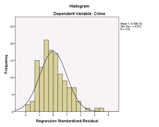
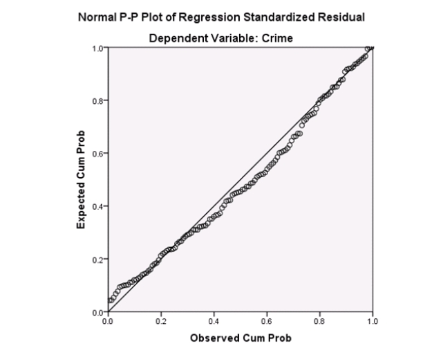 The explanatory variables tuition,age,and liquor not highly corrected with crime.Does that mean they should not be in the model?
A)Yes,because only variables that are highly correlated with the response variable will be significant predictors in a regression analysis.
B)No.Just because a variable is not correlated with the response variable does not imply it will not be a statistically significant predictor.
C)No,because as long the correlation coefficient is large enough,that variable will be a significant predictor in a regression model.
D)Yes.Only in simple linear regression would variables that are not highly correlated with the response variable be statistically significant predictors in a regression model.
The explanatory variables tuition,age,and liquor not highly corrected with crime.Does that mean they should not be in the model?A)Yes,because only variables that are highly correlated with the response variable will be significant predictors in a regression analysis.
B)No.Just because a variable is not correlated with the response variable does not imply it will not be a statistically significant predictor.
C)No,because as long the correlation coefficient is large enough,that variable will be a significant predictor in a regression model.
D)Yes.Only in simple linear regression would variables that are not highly correlated with the response variable be statistically significant predictors in a regression model.
Question
Many people believe that parents' marital status influences their child's development throughout life and has a large effect on their child's skill in sports.A survey was sent to 100 students who were in athletics in college.Responses from 35 students were received.The researchers were interested in determining whether the marital status and level of happiness of the students' parents would predict the student's self-rated skill level in a sport.The statistical model for the multiple linear regression is in the form of which of the following? (Note: assume i = 1 to n,where n is the number of cases. )
A)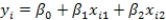

B)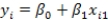

C)

D)

A)
B)
C)
D)
Question
Question
Campus crime rates are generally lower than the national average;however thousands of crimes take place on college campuses daily.Cities that are notoriously dangerous would likely be undesirable locations for a college campus.A study examined the crime rates on campuses throughout the United States and whether or not they were significantly affected by surrounding cities.A regression analysis was performed to investigate which characteristics of a city,along with a few chosen demographics of a school,impacted the crime rate on a college campus.There are over 4000 colleges and universities in the United States.The study included a random sample of 129 institutions.The response variable was the number of crimes per 1000 people.Explanatory variables included the percent of married couples in the city (married),tuition of the university (tuition),average income of the city (income),unemployment rate of the city (unemployment),percent of students who belong to a fraternity or sorority (Greek),average age of the students at the university (age),and number of liquor stores in the city (liquor).A complete analysis of the data is shown below. 


 Does the response variable,crime,meet the assumption necessary for the analysis?
A)Yes,the response variable appears perfectly normal.
B)No,the Q-Q plot shows slight curvatures which may indicate the data are skewed.
C)You cannot tell from the information provided.
D)There are no assumptions for the response variable for a regression analysis.
Does the response variable,crime,meet the assumption necessary for the analysis?A)Yes,the response variable appears perfectly normal.
B)No,the Q-Q plot shows slight curvatures which may indicate the data are skewed.
C)You cannot tell from the information provided.
D)There are no assumptions for the response variable for a regression analysis.
Question
Campus crime rates are generally lower than the national average;however thousands of crimes take place on college campuses daily.Cities that are notoriously dangerous would likely be undesirable locations for a college campus.A study examined the crime rates on campuses throughout the United States and whether or not they were significantly affected by surrounding cities.A regression analysis was performed to investigate which characteristics of a city,along with a few chosen demographics of a school,impacted the crime rate on a college campus.There are over 4000 colleges and universities in the United States.The study included a random sample of 129 institutions.The response variable was the number of crimes per 1000 people.Explanatory variables included the percent of married couples in the city (married),tuition of the university (tuition),average income of the city (income),unemployment rate of the city (unemployment),percent of students who belong to a fraternity or sorority (Greek),average age of the students at the university (age),and number of liquor stores in the city (liquor).A complete analysis of the data is shown below. 


 What type of statistical analysis was used on these data?
A)Simple linear regression
B)Multiple linear regression
C)Logistic regression
D)Categorical data analysis
What type of statistical analysis was used on these data?A)Simple linear regression
B)Multiple linear regression
C)Logistic regression
D)Categorical data analysis
Question
Campus crime rates are generally lower than the national average;however thousands of crimes take place on college campuses daily.Cities that are notoriously dangerous would likely be undesirable locations for a college campus.A study examined the crime rates on campuses throughout the United States and whether or not they were significantly affected by surrounding cities.A regression analysis was performed to investigate which characteristics of a city,along with a few chosen demographics of a school,impacted the crime rate on a college campus.There are over 4000 colleges and universities in the United States.The study included a random sample of 129 institutions.The response variable was the number of crimes per 1000 people.Explanatory variables included the percent of married couples in the city (married),tuition of the university (tuition),average income of the city (income),unemployment rate of the city (unemployment),percent of students who belong to a fraternity or sorority (Greek),average age of the students at the university (age),and number of liquor stores in the city (liquor).A complete analysis of the data is shown below. 


 The ANOVA F statistic is 1.642 with a P-value of .130.What does this tell us about the regression coefficients for the explanatory variables?
A)At least one of the regression coefficients is different from zero in the population regression equation.
B)All of the regression coefficients are different from zero in the population regression equation.
C)None of the regression coefficients are different from zero in the population regression equation.
The ANOVA F statistic is 1.642 with a P-value of .130.What does this tell us about the regression coefficients for the explanatory variables?A)At least one of the regression coefficients is different from zero in the population regression equation.
B)All of the regression coefficients are different from zero in the population regression equation.
C)None of the regression coefficients are different from zero in the population regression equation.
Question
Question
Campus crime rates are generally lower than the national average;however thousands of crimes take place on college campuses daily.Cities that are notoriously dangerous would likely be undesirable locations for a college campus.A study examined the crime rates on campuses throughout the United States and whether or not they were significantly affected by surrounding cities.A regression analysis was performed to investigate which characteristics of a city,along with a few chosen demographics of a school,impacted the crime rate on a college campus.There are over 4000 colleges and universities in the United States.The study included a random sample of 129 institutions.The response variable was the number of crimes per 1000 people.Explanatory variables included the percent of married couples in the city (married),tuition of the university (tuition),average income of the city (income),unemployment rate of the city (unemployment),percent of students who belong to a fraternity or sorority (Greek),average age of the students at the university (age),and number of liquor stores in the city (liquor).A complete analysis of the data is shown below. 


 Does the significance test for the individual regression coefficients for marriage and income contradict the information we obtained from the correlation table?
A)Yes,both marriage and income are correlated with crime and the correlation is statistically significant.Therefore,something is wrong with the regression analysis.
B)No,marriage and income are both highly correlated with each other.Therefore,there is likely a significant overlap of the predictive information from these variables.
Does the significance test for the individual regression coefficients for marriage and income contradict the information we obtained from the correlation table?A)Yes,both marriage and income are correlated with crime and the correlation is statistically significant.Therefore,something is wrong with the regression analysis.
B)No,marriage and income are both highly correlated with each other.Therefore,there is likely a significant overlap of the predictive information from these variables.

Unlock Deck
Sign up to unlock the cards in this deck!
Unlock Deck
Unlock Deck
1/95
Play
Full screen (f)
Deck 11: Multiple Regression
1
A researcher is investigating possible explanations for deaths in traffic accidents.He examined data from 1991 for each of the 50 states plus Washington,DC.The data included information on the following variables. As part of his investigation he ran the multiple regression model, Deaths = 0 + 1(Children)+ 2(Income)+ i,
Where the deviations i were assumed to be independent and Normally distributed with a mean of 0 and a standard deviation of .This model was fit to the data using the method of least squares.The following results were obtained from statistical software. The researcher also ran the simple linear regression model
Deaths = 0 + 2(Income)+ i.
The following results were obtained from statistical software: What is the value of R2 in the simple linear regression model?
A)0.014
B)0.020
C)0.688
D)0.941
As part of his investigation he ran the multiple regression model, Deaths = 0 + 1(Children)+ 2(Income)+ i,Where the deviations i were assumed to be independent and Normally distributed with a mean of 0 and a standard deviation of .This model was fit to the data using the method of least squares.The following results were obtained from statistical software.
The researcher also ran the simple linear regression modelDeaths = 0 + 2(Income)+ i.
The following results were obtained from statistical software:
What is the value of R2 in the simple linear regression model?A)0.014
B)0.020
C)0.688
D)0.941
0.014
2
A researcher is investigating possible explanations for deaths in traffic accidents.He examined data from 1991 for each of the 50 states plus Washington,DC.The data included information on the following variables. As part of his investigation he ran the multiple regression model, Deaths = 0 + 1(Children)+ 2(Income)+ i,
Where the deviations i were assumed to be independent and Normally distributed with a mean of 0 and a standard deviation of .This model was fit to the data using the method of least squares.The following results were obtained from statistical software. Suppose we wish to test the hypotheses H0: 1 = 2 = 0 versus Ha: at least one of the j is not 0 using the ANOVA F test.What can we say about the P-value for the ANOVA F test?
A)P-value < 0.001
B)0.001C)0.005 D)P-value > 0.01
As part of his investigation he ran the multiple regression model, Deaths = 0 + 1(Children)+ 2(Income)+ i,Where the deviations i were assumed to be independent and Normally distributed with a mean of 0 and a standard deviation of .This model was fit to the data using the method of least squares.The following results were obtained from statistical software.
Suppose we wish to test the hypotheses H0: 1 = 2 = 0 versus Ha: at least one of the j is not 0 using the ANOVA F test.What can we say about the P-value for the ANOVA F test?A)P-value < 0.001
B)0.001
P-value < 0.001
3
Based on a sample of the salaries of professors at a major university,you have performed a multiple linear regression relating salary to years of service and gender.The data included information on the following variables. The estimated multiple linear regression model is Salary = 45 + 3(Years)+ 4(Gender)+ 1(Years)(Gender).
Using the multiple linear regression equation,what would you estimate the average difference in the salaries of a male professor with 3 years of service and a female professor with 3 years of service to be?
A)$3000
B)$4000
C)$5000
D)$7000
The estimated multiple linear regression model is Salary = 45 + 3(Years)+ 4(Gender)+ 1(Years)(Gender).Using the multiple linear regression equation,what would you estimate the average difference in the salaries of a male professor with 3 years of service and a female professor with 3 years of service to be?
A)$3000
B)$4000
C)$5000
D)$7000
$7000
4
A researcher is investigating possible explanations for deaths in traffic accidents.He examined data from 1991 for each of the 50 states plus Washington,DC.The data included information on the following variables. As part of his investigation he ran the multiple regression model, Deaths = 0 + 1(Children)+ 2(Income)+ i,
Where the deviations i were assumed to be independent and Normally distributed with a mean of 0 and a standard deviation of .This model was fit to the data using the method of least squares.The following results were obtained from statistical software. The researcher also ran the simple linear regression model
Deaths = 0 + 2(Income)+ i.
The following results were obtained from statistical software: Based on the above results,the researcher tested the hypotheses H0: 2 = 0 versus Ha: 2 0.What do we know about the P-value of the test?
A)P-value < 0.025
B)0.025
C)0.05
D)P-value > 0.10
As part of his investigation he ran the multiple regression model, Deaths = 0 + 1(Children)+ 2(Income)+ i,Where the deviations i were assumed to be independent and Normally distributed with a mean of 0 and a standard deviation of .This model was fit to the data using the method of least squares.The following results were obtained from statistical software.
The researcher also ran the simple linear regression modelDeaths = 0 + 2(Income)+ i.
The following results were obtained from statistical software:
Based on the above results,the researcher tested the hypotheses H0: 2 = 0 versus Ha: 2 0.What do we know about the P-value of the test?A)P-value < 0.025
B)0.025
C)0.05
D)P-value > 0.10
Unlock Deck
Unlock for access to all 95 flashcards in this deck.
Unlock Deck
k this deck
5
In a multiple regression with three explanatory variables,the total sum of squares SST = 1008,the model mean square MSM = 76,and the test statistic F = 2.533.How many observations were used?
A)26
B)29
C)30
D)31
A)26
B)29
C)30
D)31
Unlock Deck
Unlock for access to all 95 flashcards in this deck.
Unlock Deck
k this deck
6
In a multiple regression with two explanatory variables,the total sum of squares SST = 1000 and the mean square error MSE = 40.There are 13 observations.What is the value of R2?
A)0.04
B)0.52
C)0.60
D)0.96
A)0.04
B)0.52
C)0.60
D)0.96
Unlock Deck
Unlock for access to all 95 flashcards in this deck.
Unlock Deck
k this deck
7
The data referred to in this question were collected from several sales districts across the country.The data represent sales for a maker of asphalt roofing shingles.Information on the following variables is available. Partial SPSS regression output of a multiple regression model with sales as the response variable and the other four variables as predictor variables are given below. What is a 95% confidence interval for the coefficient of promotional expenditures?
A)(-0.441,4.055)
B)(-0.312,3.926)
C)(-0.053,3.667)
D)(0.726,2.888)
Partial SPSS regression output of a multiple regression model with sales as the response variable and the other four variables as predictor variables are given below. What is a 95% confidence interval for the coefficient of promotional expenditures?A)(-0.441,4.055)
B)(-0.312,3.926)
C)(-0.053,3.667)
D)(0.726,2.888)
Unlock Deck
Unlock for access to all 95 flashcards in this deck.
Unlock Deck
k this deck
8
The data referred to in this question were collected from several sales districts across the country.The data represent sales for a maker of asphalt roofing shingles.Information on the following variables is available. Partial SPSS regression output of a multiple regression model with sales as the response variable and the other four variables as predictor variables are given below. What is the estimate for the error variance 2?
A)9.604
B)12.960
C)92.245
D)1937.137
Partial SPSS regression output of a multiple regression model with sales as the response variable and the other four variables as predictor variables are given below. What is the estimate for the error variance 2?A)9.604
B)12.960
C)92.245
D)1937.137
Unlock Deck
Unlock for access to all 95 flashcards in this deck.
Unlock Deck
k this deck
9
The data referred to in this question were collected from several sales districts across the country.The data represent sales for a maker of asphalt roofing shingles.Information on the following variables is available. Partial SPSS regression output of a multiple regression model with sales as the response variable and the other four variables as predictor variables are given below. In an attempt to increase sales,the company can only directly influence some of these variables.It cannot change the number of competitors;it cannot change the district potential.The only two variables they can actively change are the number of active accounts and the promotional expenditures.Suppose they have $5000 to spend on new commercials (that is,promotional expenditures).By how much are sales expected to increase?
A)1.807 squares
B)9.035 squares
C)1807 squares
D)9035 squares
Partial SPSS regression output of a multiple regression model with sales as the response variable and the other four variables as predictor variables are given below. In an attempt to increase sales,the company can only directly influence some of these variables.It cannot change the number of competitors;it cannot change the district potential.The only two variables they can actively change are the number of active accounts and the promotional expenditures.Suppose they have $5000 to spend on new commercials (that is,promotional expenditures).By how much are sales expected to increase?A)1.807 squares
B)9.035 squares
C)1807 squares
D)9035 squares
Unlock Deck
Unlock for access to all 95 flashcards in this deck.
Unlock Deck
k this deck
10
A researcher is investigating possible explanations for deaths in traffic accidents.He examined data from 1991 for each of the 50 states plus Washington,DC.The data included information on the following variables. As part of his investigation he ran the multiple regression model, Deaths = 0 + 1(Children)+ 2(Income)+ i,
Where the deviations i were assumed to be independent and Normally distributed with a mean of 0 and a standard deviation of .This model was fit to the data using the method of least squares.The following results were obtained from statistical software. The researcher also ran the simple linear regression model
Deaths = 0 + 2(Income)+ i.
The following results were obtained from statistical software: Based on the analyses,what can we conclude?
A)The variable income is statistically significant at level 0.05 as a predictor of the variable deaths.
B)The variable income is statistically significant at level 0.05 as a predictor of the variable deaths in a multiple regression model that includes the variable children.
C)The variable income is not useful as a predictor of the variable deaths and should be omitted from the analysis.
D)The variable children is not useful as a predictor of the variable deaths,unless the variable income is also present in the multiple regression model.
As part of his investigation he ran the multiple regression model, Deaths = 0 + 1(Children)+ 2(Income)+ i,Where the deviations i were assumed to be independent and Normally distributed with a mean of 0 and a standard deviation of .This model was fit to the data using the method of least squares.The following results were obtained from statistical software.
The researcher also ran the simple linear regression modelDeaths = 0 + 2(Income)+ i.
The following results were obtained from statistical software:
Based on the analyses,what can we conclude?A)The variable income is statistically significant at level 0.05 as a predictor of the variable deaths.
B)The variable income is statistically significant at level 0.05 as a predictor of the variable deaths in a multiple regression model that includes the variable children.
C)The variable income is not useful as a predictor of the variable deaths and should be omitted from the analysis.
D)The variable children is not useful as a predictor of the variable deaths,unless the variable income is also present in the multiple regression model.
Unlock Deck
Unlock for access to all 95 flashcards in this deck.
Unlock Deck
k this deck
11
A researcher is investigating possible explanations for deaths in traffic accidents.He examined data from 1991 for each of the 50 states plus Washington,DC.The data included information on the following variables. As part of his investigation he ran the multiple regression model, Deaths = 0 + 1(Children)+ 2(Income)+ i,
Where the deviations i were assumed to be independent and Normally distributed with a mean of 0 and a standard deviation of .This model was fit to the data using the method of least squares.The following results were obtained from statistical software. The researcher also ran the simple linear regression model
Deaths = 0 + 2(Income)+ i.
The following results were obtained from statistical software: What can we conclude regarding the meaningfulness of the analyses?
A)They are very meaningful because the results are based on a very large sample consisting of the people in all 50 states as well as Washington,DC.
B)They are meaningful because R2 for the multiple regression model is quite large,suggesting that the model fits well and the assumptions about the model are reasonable.
C)They are moderately meaningful because the results are based on a fairly large sample and they are at least consistent with what one would expect.They would be very meaningful if,in addition,we had examined the residuals and found no outliers or influential observations.
D)They are not necessarily meaningful because these results are based on available data.
As part of his investigation he ran the multiple regression model, Deaths = 0 + 1(Children)+ 2(Income)+ i,Where the deviations i were assumed to be independent and Normally distributed with a mean of 0 and a standard deviation of .This model was fit to the data using the method of least squares.The following results were obtained from statistical software.
The researcher also ran the simple linear regression modelDeaths = 0 + 2(Income)+ i.
The following results were obtained from statistical software:
What can we conclude regarding the meaningfulness of the analyses?A)They are very meaningful because the results are based on a very large sample consisting of the people in all 50 states as well as Washington,DC.
B)They are meaningful because R2 for the multiple regression model is quite large,suggesting that the model fits well and the assumptions about the model are reasonable.
C)They are moderately meaningful because the results are based on a fairly large sample and they are at least consistent with what one would expect.They would be very meaningful if,in addition,we had examined the residuals and found no outliers or influential observations.
D)They are not necessarily meaningful because these results are based on available data.
Unlock Deck
Unlock for access to all 95 flashcards in this deck.
Unlock Deck
k this deck
12
In a multiple regression with four explanatory variables,data are collected on 25 observations.What is the largest value the ANOVA F statistic can take on before we would reject the null hypothesis that all of the regression coefficients are zero,at the 5% significance level?
A)2.78
B)2.87
C)3.10
D)3.51
A)2.78
B)2.87
C)3.10
D)3.51
Unlock Deck
Unlock for access to all 95 flashcards in this deck.
Unlock Deck
k this deck
13
What proportion of the variation in the variable deaths is explained by the explanatory variables children and income?
A)0.059
B)0.159
C)0.470
D)0.941
A)0.059
B)0.159
C)0.470
D)0.941
Unlock Deck
Unlock for access to all 95 flashcards in this deck.
Unlock Deck
k this deck
14
In a multiple regression with five explanatory variables,data are collected on 63 observations.What are the degrees of freedom for the ANOVA F test?
A)4 and 57
B)5 and 57
C)5 and 58
D)5 and 62
A)4 and 57
B)5 and 57
C)5 and 58
D)5 and 62
Unlock Deck
Unlock for access to all 95 flashcards in this deck.
Unlock Deck
k this deck
15
A researcher is investigating possible explanations for deaths in traffic accidents.He examined data from 1991 for each of the 50 states plus Washington,DC.The data included information on the following variables. As part of his investigation he ran the multiple regression model, Deaths = 0 + 1(Children)+ 2(Income)+ i,
Where the deviations i were assumed to be independent and Normally distributed with a mean of 0 and a standard deviation of .This model was fit to the data using the method of least squares.The following results were obtained from statistical software. Suppose we wish to test the hypotheses H0: 1 = 2 = 0 versus Ha: at least one of the j is not 0 using the ANOVA F test.What is the value of the F statistic?
A)0.94
B)15.9
C)24
D)381.5
As part of his investigation he ran the multiple regression model, Deaths = 0 + 1(Children)+ 2(Income)+ i,Where the deviations i were assumed to be independent and Normally distributed with a mean of 0 and a standard deviation of .This model was fit to the data using the method of least squares.The following results were obtained from statistical software.
Suppose we wish to test the hypotheses H0: 1 = 2 = 0 versus Ha: at least one of the j is not 0 using the ANOVA F test.What is the value of the F statistic?A)0.94
B)15.9
C)24
D)381.5
Unlock Deck
Unlock for access to all 95 flashcards in this deck.
Unlock Deck
k this deck
16
The data referred to in this question were collected from several sales districts across the country.The data represent sales for a maker of asphalt roofing shingles.Information on the following variables is available. Partial SPSS regression output of a multiple regression model with sales as the response variable and the other four variables as predictor variables are given below. What proportion of the variation in sales is explained by the set of all four explanatory variables?
A)-0.647
B)0.558
C)0.989
D)0.995
Partial SPSS regression output of a multiple regression model with sales as the response variable and the other four variables as predictor variables are given below. What proportion of the variation in sales is explained by the set of all four explanatory variables?A)-0.647
B)0.558
C)0.989
D)0.995
Unlock Deck
Unlock for access to all 95 flashcards in this deck.
Unlock Deck
k this deck
17
The data referred to in this question were collected from several sales districts across the country.The data represent sales for a maker of asphalt roofing shingles.Information on the following variables is available. Partial SPSS regression output of a multiple regression model with sales as the response variable and the other four variables as predictor variables are given below. Which of the four explanatory variables seems to be the least significant in the model?
A)Expenditures
B)Accounts
C)Competing brands
D)District potential
Partial SPSS regression output of a multiple regression model with sales as the response variable and the other four variables as predictor variables are given below. Which of the four explanatory variables seems to be the least significant in the model?A)Expenditures
B)Accounts
C)Competing brands
D)District potential
Unlock Deck
Unlock for access to all 95 flashcards in this deck.
Unlock Deck
k this deck
18
A researcher is investigating possible explanations for deaths in traffic accidents.He examined data from 1991 for each of the 50 states plus Washington,DC.The data included information on the following variables. As part of his investigation he ran the multiple regression model, Deaths = 0 + 1(Children)+ 2(Income)+ i,
Where the deviations i were assumed to be independent and Normally distributed with a mean of 0 and a standard deviation of .This model was fit to the data using the method of least squares.The following results were obtained from statistical software. What is a 99% confidence interval for 2,the coefficient of the variable income?
A)-0.039 ± 0.030
B)-0.039 ± 0.040
C)0.015 ± 0.079
D)0.015 ± 0.104
As part of his investigation he ran the multiple regression model, Deaths = 0 + 1(Children)+ 2(Income)+ i,Where the deviations i were assumed to be independent and Normally distributed with a mean of 0 and a standard deviation of .This model was fit to the data using the method of least squares.The following results were obtained from statistical software.
What is a 99% confidence interval for 2,the coefficient of the variable income?A)-0.039 ± 0.030
B)-0.039 ± 0.040
C)0.015 ± 0.079
D)0.015 ± 0.104
Unlock Deck
Unlock for access to all 95 flashcards in this deck.
Unlock Deck
k this deck
19
The data referred to in this question were collected from several sales districts across the country.The data represent sales for a maker of asphalt roofing shingles.Information on the following variables is available. Partial SPSS regression output of a multiple regression model with sales as the response variable and the other four variables as predictor variables are given below. An F test for the two coefficients of promotional expenditures and district potential is performed.The hypotheses are H0: 1 = 4 = 0 versus Ha: at least one of the j is not 0.The F statistic for this test is 1.482 with 2 and 21 degrees of freedom.What can we say about the P-value for this test?
A)P-value < 0.025
B)0.025
C)0.05
D)P-value > 0.10
Partial SPSS regression output of a multiple regression model with sales as the response variable and the other four variables as predictor variables are given below. An F test for the two coefficients of promotional expenditures and district potential is performed.The hypotheses are H0: 1 = 4 = 0 versus Ha: at least one of the j is not 0.The F statistic for this test is 1.482 with 2 and 21 degrees of freedom.What can we say about the P-value for this test?A)P-value < 0.025
B)0.025
C)0.05
D)P-value > 0.10
Unlock Deck
Unlock for access to all 95 flashcards in this deck.
Unlock Deck
k this deck
20
The data referred to in this question were collected from several sales districts across the country.The data represent sales for a maker of asphalt roofing shingles.Information on the following variables is available. Partial SPSS regression output of a multiple regression model with sales as the response variable and the other four variables as predictor variables are given below. How many districts were sampled in all?
A)21
B)24
C)25
D)26
Partial SPSS regression output of a multiple regression model with sales as the response variable and the other four variables as predictor variables are given below. How many districts were sampled in all?A)21
B)24
C)25
D)26
Unlock Deck
Unlock for access to all 95 flashcards in this deck.
Unlock Deck
k this deck
21
Researchers at a large nutrition and weight management company are trying to build a model to predict a person's body fat percentage from an array of variables such as body weight,height,and body measurements around the neck,chest,abdomen,hips,biceps,etc.A variable selection method is used to build a simple model.SPSS output for the final model is given below. A graph of the residuals versus the predicted values is given below. What assumption do we check with this graph?
A)The Normality of the error terms
B)The independence of the residuals
C)The constant variance assumption of the predicted values
D)None of the above
A graph of the residuals versus the predicted values is given below. What assumption do we check with this graph?A)The Normality of the error terms
B)The independence of the residuals
C)The constant variance assumption of the predicted values
D)None of the above
Unlock Deck
Unlock for access to all 95 flashcards in this deck.
Unlock Deck
k this deck
22
A researcher is investigating variables that might be associated with the academic performance of high school students.She examined data from 1990 for each of the 50 states plus Washington,DC.The data included information on the following variables. As part of her investigation,she ran the multiple regression model SATM = 0 + 1($ per pupil)+ 2(% taking)+ i,
Where the deviations i were assumed to be independent and Normally distributed with a mean of 0 and a standard deviation of .This model was fit to the data using the method of least squares.The following results were obtained from statistical software. Suppose we wish to test the hypotheses H0: 1 = 2 = 0 versus Ha: at least one of the j is not 0,using the ANOVA F test.What is the value of the F statistic?
A)3.32
B)24.0
C)79.65
D)159.3
As part of her investigation,she ran the multiple regression model SATM = 0 + 1($ per pupil)+ 2(% taking)+ i,Where the deviations i were assumed to be independent and Normally distributed with a mean of 0 and a standard deviation of .This model was fit to the data using the method of least squares.The following results were obtained from statistical software.
Suppose we wish to test the hypotheses H0: 1 = 2 = 0 versus Ha: at least one of the j is not 0,using the ANOVA F test.What is the value of the F statistic?A)3.32
B)24.0
C)79.65
D)159.3
Unlock Deck
Unlock for access to all 95 flashcards in this deck.
Unlock Deck
k this deck
23
Researchers at a car resale company are trying to build a model to predict a car's 4-year resale value (in thousands of dollars)from several predictor variables.The variables they selected are as below. Data were collected on cars of different models made by different manufacturers.SPSS output for the least-squares regression model is given below. A Normal quantile plot of the residuals is given below. What assumption do we check with this graph,and does the assumption seem to be satisfied?
Data were collected on cars of different models made by different manufacturers.SPSS output for the least-squares regression model is given below. A Normal quantile plot of the residuals is given below. What assumption do we check with this graph,and does the assumption seem to be satisfied? Unlock Deck
Unlock for access to all 95 flashcards in this deck.
Unlock Deck
k this deck
24
Based on a sample of the salaries of professors at a major university,you have performed a multiple linear regression relating salary to years of service and gender.The data included information on the following variables. The estimated multiple linear regression model is Salary = 45 + 3(Years)+ 4(Gender)+ 1(Years)(Gender).
A particular female professor with 6 years of experience currently has a salary of $60,000.What is the residual for this observation?
A)-$9000
B)-$3000
C)$3000
D)$9000
The estimated multiple linear regression model is Salary = 45 + 3(Years)+ 4(Gender)+ 1(Years)(Gender).A particular female professor with 6 years of experience currently has a salary of $60,000.What is the residual for this observation?
A)-$9000
B)-$3000
C)$3000
D)$9000
Unlock Deck
Unlock for access to all 95 flashcards in this deck.
Unlock Deck
k this deck
25
A researcher is investigating variables that might be associated with the academic performance of high school students.She examined data from 1990 for each of the 50 states plus Washington,DC.The data included information on the following variables. As part of her investigation,she ran the multiple regression model SATM = 0 + 1($ per pupil)+ 2(% taking)+ i,
Where the deviations i were assumed to be independent and Normally distributed with a mean of 0 and a standard deviation of .This model was fit to the data using the method of least squares.The following results were obtained from statistical software. What proportion of the variation in the variable SATM is explained by the explanatory variables $ per pupil and % taking?
A)0.232
B)0.301
C)0.768
D)0.960
As part of her investigation,she ran the multiple regression model SATM = 0 + 1($ per pupil)+ 2(% taking)+ i,Where the deviations i were assumed to be independent and Normally distributed with a mean of 0 and a standard deviation of .This model was fit to the data using the method of least squares.The following results were obtained from statistical software.
What proportion of the variation in the variable SATM is explained by the explanatory variables $ per pupil and % taking?A)0.232
B)0.301
C)0.768
D)0.960
Unlock Deck
Unlock for access to all 95 flashcards in this deck.
Unlock Deck
k this deck
26
A researcher is investigating variables that might be associated with the academic performance of high school students.She examined data from 1990 for each of the 50 states plus Washington,DC.The data included information on the following variables. As part of her investigation,she ran the multiple regression model SATM = 0 + 1($ per pupil)+ 2(% taking)+ i,
Where the deviations i were assumed to be independent and Normally distributed with a mean of 0 and a standard deviation of .This model was fit to the data using the method of least squares.The following results were obtained from statistical software. Another researcher,using the same data,ran the simple linear regression model
SATM = 0 + 1($ per pupil)+ i.
The following results were obtained from statistical software. The first researcher concluded that because the coefficient for the variable $ per pupil was positive in her results,spending additional money on students would have a positive effect on SATM scores.This researcher therefore recommended more money be spent on students.The second researcher concluded that because the coefficient for the variable $ per pupil was negative in his results,spending additional money on students would have a negative effect on SATM scores.This researcher therefore recommended less money be spent on students.Why are these two conclusions different even though the researchers used the same data?
A)An error must have been made by one of the researchers.
B)Both researchers failed to take into account that in their analyses,1,the coefficient of the variable $ per pupil,was not statistically significant at even the 0.10 significance level.Hence,neither researcher could conclude that 1 was significantly different from zero.
C)The researchers did not use the same set of explanatory variables in their models.
D)There must have been an influential observation in the data,rendering the analyses inappropriate.
As part of her investigation,she ran the multiple regression model SATM = 0 + 1($ per pupil)+ 2(% taking)+ i,Where the deviations i were assumed to be independent and Normally distributed with a mean of 0 and a standard deviation of .This model was fit to the data using the method of least squares.The following results were obtained from statistical software.
Another researcher,using the same data,ran the simple linear regression modelSATM = 0 + 1($ per pupil)+ i.
The following results were obtained from statistical software.
The first researcher concluded that because the coefficient for the variable $ per pupil was positive in her results,spending additional money on students would have a positive effect on SATM scores.This researcher therefore recommended more money be spent on students.The second researcher concluded that because the coefficient for the variable $ per pupil was negative in his results,spending additional money on students would have a negative effect on SATM scores.This researcher therefore recommended less money be spent on students.Why are these two conclusions different even though the researchers used the same data?A)An error must have been made by one of the researchers.
B)Both researchers failed to take into account that in their analyses,1,the coefficient of the variable $ per pupil,was not statistically significant at even the 0.10 significance level.Hence,neither researcher could conclude that 1 was significantly different from zero.
C)The researchers did not use the same set of explanatory variables in their models.
D)There must have been an influential observation in the data,rendering the analyses inappropriate.
Unlock Deck
Unlock for access to all 95 flashcards in this deck.
Unlock Deck
k this deck
27
Researchers at a car resale company are trying to build a model to predict a car's 4-year resale value (in thousands of dollars)from several predictor variables.The variables they selected are as below. Data were collected on cars of different models made by different manufacturers.SPSS output for the least-squares regression model is given below. A particular car (not a truck)cost $40,000 and has an engine of 3.8 liters.What do you predict the 4-year resale value of this car to be?
Data were collected on cars of different models made by different manufacturers.SPSS output for the least-squares regression model is given below. A particular car (not a truck)cost $40,000 and has an engine of 3.8 liters.What do you predict the 4-year resale value of this car to be? Unlock Deck
Unlock for access to all 95 flashcards in this deck.
Unlock Deck
k this deck
28
Researchers at a large nutrition and weight management company are trying to build a model to predict a person's body fat percentage from an array of variables such as body weight,height,and body measurements around the neck,chest,abdomen,hips,biceps,etc.A variable selection method is used to build a simple model.SPSS output for the final model is given below. What percentage of the variation in percent body fat remains unexplained,even after introducing weight and abdomen circumference into the model?
A)7.86%
B)15.11%
C)84.89%
D)92.14%
What percentage of the variation in percent body fat remains unexplained,even after introducing weight and abdomen circumference into the model?A)7.86%
B)15.11%
C)84.89%
D)92.14%
Unlock Deck
Unlock for access to all 95 flashcards in this deck.
Unlock Deck
k this deck
29
Researchers at a car resale company are trying to build a model to predict a car's 4-year resale value (in thousands of dollars)from several predictor variables.The variables they selected are as below. Data were collected on cars of different models made by different manufacturers.SPSS output for the least-squares regression model is given below. Suppose we wish to test the hypotheses H0: 1 = 0 versus Ha: 1 0,where 1 is the coefficient for the variable type.Based on the 95% confidence interval given in the output,what do we know about the value of the P-value of this test?
Data were collected on cars of different models made by different manufacturers.SPSS output for the least-squares regression model is given below. Suppose we wish to test the hypotheses H0: 1 = 0 versus Ha: 1 0,where 1 is the coefficient for the variable type.Based on the 95% confidence interval given in the output,what do we know about the value of the P-value of this test? Unlock Deck
Unlock for access to all 95 flashcards in this deck.
Unlock Deck
k this deck
30
Based on a sample of the salaries of professors at a major university,you have performed a multiple linear regression relating salary to years of service and gender.The data included information on the following variables. The estimated multiple linear regression model is Salary = 45 + 3(Years)+ 4(Gender)+ 1(Years)(Gender).
Using the multiple linear regression equation,what would you estimate the average salary of male professors with 3 years of experience to be?
A)$53,000
B)$54,000
C)$58,000
D)$61,000
The estimated multiple linear regression model is Salary = 45 + 3(Years)+ 4(Gender)+ 1(Years)(Gender).Using the multiple linear regression equation,what would you estimate the average salary of male professors with 3 years of experience to be?
A)$53,000
B)$54,000
C)$58,000
D)$61,000
Unlock Deck
Unlock for access to all 95 flashcards in this deck.
Unlock Deck
k this deck
31
A researcher is investigating variables that might be associated with the academic performance of high school students.She examined data from 1990 for each of the 50 states plus Washington,DC.The data included information on the following variables. As part of her investigation,she ran the multiple regression model SATM = 0 + 1($ per pupil)+ 2(% taking)+ i,
Where the deviations i were assumed to be independent and Normally distributed with a mean of 0 and a standard deviation of .This model was fit to the data using the method of least squares.The following results were obtained from statistical software. What is the value of the MSE?
A)10.30
B)288.23
C)13835.10
D)22957.50
As part of her investigation,she ran the multiple regression model SATM = 0 + 1($ per pupil)+ 2(% taking)+ i,Where the deviations i were assumed to be independent and Normally distributed with a mean of 0 and a standard deviation of .This model was fit to the data using the method of least squares.The following results were obtained from statistical software.
What is the value of the MSE?A)10.30
B)288.23
C)13835.10
D)22957.50
Unlock Deck
Unlock for access to all 95 flashcards in this deck.
Unlock Deck
k this deck
32
Researchers at a large nutrition and weight management company are trying to build a model to predict a person's body fat percentage from an array of variables such as body weight,height,and body measurements around the neck,chest,abdomen,hips,biceps,etc.A variable selection method is used to build a simple model.SPSS output for the final model is given below. How many people were included in the study?
A)46
B)48
C)49
D)50
How many people were included in the study?A)46
B)48
C)49
D)50
Unlock Deck
Unlock for access to all 95 flashcards in this deck.
Unlock Deck
k this deck
33
A researcher is investigating variables that might be associated with the academic performance of high school students.She examined data from 1990 for each of the 50 states plus Washington,DC.The data included information on the following variables. As part of her investigation,she ran the multiple regression model SATM = 0 + 1($ per pupil)+ 2(% taking)+ i,
Where the deviations i were assumed to be independent and Normally distributed with a mean of 0 and a standard deviation of .This model was fit to the data using the method of least squares.The following results were obtained from statistical software. What is an approximate 95% confidence interval for 1,the coefficient of the variable $ per pupil?
A)0.00639 ± 0.0025
B)0.00639 ± 0.0042
C)0.00639 ± 0.0050
D)0.00639 ± 0.0067
As part of her investigation,she ran the multiple regression model SATM = 0 + 1($ per pupil)+ 2(% taking)+ i,Where the deviations i were assumed to be independent and Normally distributed with a mean of 0 and a standard deviation of .This model was fit to the data using the method of least squares.The following results were obtained from statistical software.
What is an approximate 95% confidence interval for 1,the coefficient of the variable $ per pupil?A)0.00639 ± 0.0025
B)0.00639 ± 0.0042
C)0.00639 ± 0.0050
D)0.00639 ± 0.0067
Unlock Deck
Unlock for access to all 95 flashcards in this deck.
Unlock Deck
k this deck
34
A researcher is investigating variables that might be associated with the academic performance of high school students.She examined data from 1990 for each of the 50 states plus Washington,DC.The data included information on the following variables. As part of her investigation,she ran the multiple regression model SATM = 0 + 1($ per pupil)+ 2(% taking)+ i,
Where the deviations i were assumed to be independent and Normally distributed with a mean of 0 and a standard deviation of .This model was fit to the data using the method of least squares.The following results were obtained from statistical software. Another researcher,using the same data,ran the simple linear regression model
SATM = 0 + 1($ per pupil)+ i.
The following results were obtained from statistical software. Based on these results,a 95% confidence interval for 1,the coefficient of the variable $ per pupil,is approximately
A)-0.012169 ± 0.0031.
B)-0.012169 ± 0.0052.
C)-0.012169 ± 0.0062.
D)-0.012169 ± 0.0083.
As part of her investigation,she ran the multiple regression model SATM = 0 + 1($ per pupil)+ 2(% taking)+ i,Where the deviations i were assumed to be independent and Normally distributed with a mean of 0 and a standard deviation of .This model was fit to the data using the method of least squares.The following results were obtained from statistical software.
Another researcher,using the same data,ran the simple linear regression modelSATM = 0 + 1($ per pupil)+ i.
The following results were obtained from statistical software.
Based on these results,a 95% confidence interval for 1,the coefficient of the variable $ per pupil,is approximatelyA)-0.012169 ± 0.0031.
B)-0.012169 ± 0.0052.
C)-0.012169 ± 0.0062.
D)-0.012169 ± 0.0083.
Unlock Deck
Unlock for access to all 95 flashcards in this deck.
Unlock Deck
k this deck
35
Researchers at a large nutrition and weight management company are trying to build a model to predict a person's body fat percentage from an array of variables such as body weight,height,and body measurements around the neck,chest,abdomen,hips,biceps,etc.A variable selection method is used to build a simple model.SPSS output for the final model is given below. What is a 90% confidence interval for 1,the coefficient of weight,based on these results?
A)-0.162 ± 0.038
B)-0.162 ± 0.064
C)-0.162 ± 0.525
D)-0.162 ± 4.230
What is a 90% confidence interval for 1,the coefficient of weight,based on these results?A)-0.162 ± 0.038
B)-0.162 ± 0.064
C)-0.162 ± 0.525
D)-0.162 ± 4.230
Unlock Deck
Unlock for access to all 95 flashcards in this deck.
Unlock Deck
k this deck
36
Researchers at a car resale company are trying to build a model to predict a car's 4-year resale value (in thousands of dollars)from several predictor variables.The variables they selected are as below. Data were collected on cars of different models made by different manufacturers.SPSS output for the least-squares regression model is given below. An F test for the two coefficients of type and engine is performed.The hypotheses areH0: 1 = 3 = 0 versus Ha: at least one of the j is not 0.The F statistic for this test is 12.21 with 2 and 115 degrees of freedom.Do we reject the null hypothesis at the 5% significance level?
Data were collected on cars of different models made by different manufacturers.SPSS output for the least-squares regression model is given below. An F test for the two coefficients of type and engine is performed.The hypotheses areH0: 1 = 3 = 0 versus Ha: at least one of the j is not 0.The F statistic for this test is 12.21 with 2 and 115 degrees of freedom.Do we reject the null hypothesis at the 5% significance level? Unlock Deck
Unlock for access to all 95 flashcards in this deck.
Unlock Deck
k this deck
37
Researchers at a car resale company are trying to build a model to predict a car's 4-year resale value (in thousands of dollars)from several predictor variables.The variables they selected are as below. Data were collected on cars of different models made by different manufacturers.SPSS output for the least-squares regression model is given below. What is the equation of the least-squares regression line?
Data were collected on cars of different models made by different manufacturers.SPSS output for the least-squares regression model is given below. What is the equation of the least-squares regression line? Unlock Deck
Unlock for access to all 95 flashcards in this deck.
Unlock Deck
k this deck
38
Researchers at a large nutrition and weight management company are trying to build a model to predict a person's body fat percentage from an array of variables such as body weight,height,and body measurements around the neck,chest,abdomen,hips,biceps,etc.A variable selection method is used to build a simple model.SPSS output for the final model is given below. What is the value of an estimate of 2?
A)3.4369
B)11.813
C)543.379
D)1526.645
What is the value of an estimate of 2?A)3.4369
B)11.813
C)543.379
D)1526.645
Unlock Deck
Unlock for access to all 95 flashcards in this deck.
Unlock Deck
k this deck
39
Researchers at a large nutrition and weight management company are trying to build a model to predict a person's body fat percentage from an array of variables such as body weight,height,and body measurements around the neck,chest,abdomen,hips,biceps,etc.A variable selection method is used to build a simple model.SPSS output for the final model is given below. Suppose we wish to test the hypotheses H0: 1 = 2 = 0 versus Ha: at least one of the j is not 0,using the ANOVA F test.What is the value of the test statistic?
A)-11.379
B)-4.230
C)10.912
D)129.239
Suppose we wish to test the hypotheses H0: 1 = 2 = 0 versus Ha: at least one of the j is not 0,using the ANOVA F test.What is the value of the test statistic?A)-11.379
B)-4.230
C)10.912
D)129.239
Unlock Deck
Unlock for access to all 95 flashcards in this deck.
Unlock Deck
k this deck
40
Researchers at a car resale company are trying to build a model to predict a car's 4-year resale value (in thousands of dollars)from several predictor variables.The variables they selected are as below. Data were collected on cars of different models made by different manufacturers.SPSS output for the least-squares regression model is given below. What is the value of an estimate for the error standard deviation ?
Data were collected on cars of different models made by different manufacturers.SPSS output for the least-squares regression model is given below. What is the value of an estimate for the error standard deviation ? Unlock Deck
Unlock for access to all 95 flashcards in this deck.
Unlock Deck
k this deck
41
The NFL keeps track of a large number of statistics during the football season.For 2009 the number of points scored per game and how it related to such variables as the number of passes attempted per game (PassAtt/G),the total pass yards gained during the season (PassYds),and the total rushing yards gained in the season (RushYds)were studied.The following tables provide information on the least-squares fit of a multiple regression model for Pts/G on the three explanatory variables. What would be the 96% confidence interval estimate for the true regression coefficient for the variable PassAtt/G?
A)(-0.080,0.001)
B)(-1.025,0.007)
C)(-0.007,1.025)
D)(-5.203,4.185)
E)Not within ± 0.02 of any of the above
What would be the 96% confidence interval estimate for the true regression coefficient for the variable PassAtt/G?A)(-0.080,0.001)
B)(-1.025,0.007)
C)(-0.007,1.025)
D)(-5.203,4.185)
E)Not within ± 0.02 of any of the above
Unlock Deck
Unlock for access to all 95 flashcards in this deck.
Unlock Deck
k this deck
42
In this experiment,the risk-taking propensity of 90 inner city drug users was measured using a repeated measures test called the Behavioral Analogue Risk Task (BART;Lejuez et al. ,2002).The higher the BART score,the higher the risk-taking propensity.Participants also filled out questionnaires so that their Psychopathic Personality Inventory (PPI)scores could be computed.PPI scores are used to detect psychopathic traits in a covert manner and are a common indicator of one's level of psychopathy.The main goal of the experiment was to examine the relationship between risk-taking (measured by BART)based on one's level of psychopathy (measured by PPI on a scale of 0-100),gender (1 for male and 2 for female),and heroin use (1 for heroin use and 0 for no heroin use).Below is a partial output of a multiple regression analysis. What are the explanatory variables in this study?
A)Gender and Bart score
B)Gender and PPI
C)Gender,heroin,and PPI
What are the explanatory variables in this study?A)Gender and Bart score
B)Gender and PPI
C)Gender,heroin,and PPI
Unlock Deck
Unlock for access to all 95 flashcards in this deck.
Unlock Deck
k this deck
43
A study was conducted on 40 different brands of golf balls with respect to the distance the ball traveled after being struck with standardized test 7-iron.The response variable DIST is the measurement of the carry distance of the shot in yards.The explanatory variables are SMASH,the ratio of the ball speed/club speed at impact;SPIN,the initial spin rate of the ball in RPMs;and HEIGHT,the peak height of the ball in flight measured in feet. The following is a table showing some computer output (missing results are shown by **)for a least-squares fit of a multiple regression model using these variables. What is the value of the squared multiple correlation ?
A)0.036
B)0.960
C)0.163
D)0.964
E)0.404
What is the value of the squared multiple correlation ?A)0.036
B)0.960
C)0.163
D)0.964
E)0.404
Unlock Deck
Unlock for access to all 95 flashcards in this deck.
Unlock Deck
k this deck
44
A study was conducted on 40 different brands of golf balls with respect to the distance the ball traveled after being struck with standardized test 7-iron.The response variable DIST is the measurement of the carry distance of the shot in yards.The explanatory variables are SMASH,the ratio of the ball speed/club speed at impact;SPIN,the initial spin rate of the ball in RPMs;and HEIGHT,the peak height of the ball in flight measured in feet. The following is a table showing some computer output (missing results are shown by **)for a least-squares fit of a multiple regression model using these variables. Based upon the P-value of the ANOVA F test,what can be concluded about the relationship between the response variable and the explanatory variables?
A)A significant amount of the variation in the response variable can be explained by the regression on the explanatory variables.
B)There is strong evidence that the distance a golf ball travels depends upon the variable SMASH.
C)There is strong statistical evidence that at least one of the regression coefficients is not equal to zero.
D)When considered on its own,the variable SPIN is significantly different from zero.
E)There is strong statistical evidence that none of the regression coefficients is equal and all are significantly different from zero.
Based upon the P-value of the ANOVA F test,what can be concluded about the relationship between the response variable and the explanatory variables?A)A significant amount of the variation in the response variable can be explained by the regression on the explanatory variables.
B)There is strong evidence that the distance a golf ball travels depends upon the variable SMASH.
C)There is strong statistical evidence that at least one of the regression coefficients is not equal to zero.
D)When considered on its own,the variable SPIN is significantly different from zero.
E)There is strong statistical evidence that none of the regression coefficients is equal and all are significantly different from zero.
Unlock Deck
Unlock for access to all 95 flashcards in this deck.
Unlock Deck
k this deck
45
In this experiment,the risk-taking propensity of 90 inner city drug users was measured using a repeated measures test called the Behavioral Analogue Risk Task (BART;Lejuez et al. ,2002).The higher the BART score,the higher the risk-taking propensity.Participants also filled out questionnaires so that their Psychopathic Personality Inventory (PPI)scores could be computed.PPI scores are used to detect psychopathic traits in a covert manner and are a common indicator of one's level of psychopathy.The main goal of the experiment was to examine the relationship between risk-taking (measured by BART)based on one's level of psychopathy (measured by PPI on a scale of 0-100),gender (1 for male and 2 for female),and heroin use (1 for heroin use and 0 for no heroin use).Below is a partial output of a multiple regression analysis. What proportion of the variation of the response variable is explained by the explanatory variables?
A)4.48%
B)20%
C)2%
D)40%
What proportion of the variation of the response variable is explained by the explanatory variables?A)4.48%
B)20%
C)2%
D)40%
Unlock Deck
Unlock for access to all 95 flashcards in this deck.
Unlock Deck
k this deck
46
In this experiment,the risk-taking propensity of 90 inner city drug users was measured using a repeated measures test called the Behavioral Analogue Risk Task (BART;Lejuez et al. ,2002).The higher the BART score,the higher the risk-taking propensity.Participants also filled out questionnaires so that their Psychopathic Personality Inventory (PPI)scores could be computed.PPI scores are used to detect psychopathic traits in a covert manner and are a common indicator of one's level of psychopathy.The main goal of the experiment was to examine the relationship between risk-taking (measured by BART)based on one's level of psychopathy (measured by PPI on a scale of 0-100),gender (1 for male and 2 for female),and heroin use (1 for heroin use and 0 for no heroin use).Below is a partial output of a multiple regression analysis. Based on this model,are heroin users bigger risktakers than non-heroin users?
A)Yes
B)No
Based on this model,are heroin users bigger risktakers than non-heroin users?A)Yes
B)No
Unlock Deck
Unlock for access to all 95 flashcards in this deck.
Unlock Deck
k this deck
47
Data were obtained in a study of the oxygen uptake of 31 middle-aged-males and females while exercising.The researchers were interested in the use of a variety of variables as predictors of Oxygen Uptake.The variables that were measured on the subjects were Age,Weight,the time taken to run a specified distance (Runtime),pulse rate at the end of the run (RunPulse),their resting pulse rate (RstPulse),and their maximum pulse rate during the run (MaxPulse).The following table from a computer analysis of the data is provided (with some entries deleted and replaced by **). What is the mean square for model (MSM)?
A)144.293
B)120.244
C)721.463
D)180.366
E)141.897
What is the mean square for model (MSM)?A)144.293
B)120.244
C)721.463
D)180.366
E)141.897
Unlock Deck
Unlock for access to all 95 flashcards in this deck.
Unlock Deck
k this deck
48
In this experiment,the risk-taking propensity of 90 inner city drug users was measured using a repeated measures test called the Behavioral Analogue Risk Task (BART;Lejuez et al. ,2002).The higher the BART score,the higher the risk-taking propensity.Participants also filled out questionnaires so that their Psychopathic Personality Inventory (PPI)scores could be computed.PPI scores are used to detect psychopathic traits in a covert manner and are a common indicator of one's level of psychopathy.The main goal of the experiment was to examine the relationship between risk-taking (measured by BART)based on one's level of psychopathy (measured by PPI on a scale of 0-100),gender (1 for male and 2 for female),and heroin use (1 for heroin use and 0 for no heroin use).Below is a partial output of a multiple regression analysis. Does this model seem like an adequate model to predict risk-taking propensity?
A)No,the R-squared value is very low and most of the variables are not statistically significant.
B)Yes,the r correlation is very strong.
C)This cannot be determined from the given information.
Does this model seem like an adequate model to predict risk-taking propensity?A)No,the R-squared value is very low and most of the variables are not statistically significant.
B)Yes,the r correlation is very strong.
C)This cannot be determined from the given information.
Unlock Deck
Unlock for access to all 95 flashcards in this deck.
Unlock Deck
k this deck
49
The NFL keeps track of a large number of statistics during the football season.For 2009 the number of points scored per game and how it related to such variables as the number of passes attempted per game (PassAtt/G),the total pass yards gained during the season (PassYds),and the total rushing yards gained in the season (RushYds)were studied.The following tables provide information on the least-squares fit of a multiple regression model for Pts/G on the three explanatory variables. If a team were to attempt 30 passes per game,pass for a total of 3500 yards,and rush for 2000 yards,what would the fitted regression model predict for the points the team would score per game?
A)25.2
B)27.6
C)44.9
D)58.2
E)18.8
If a team were to attempt 30 passes per game,pass for a total of 3500 yards,and rush for 2000 yards,what would the fitted regression model predict for the points the team would score per game?A)25.2
B)27.6
C)44.9
D)58.2
E)18.8
Unlock Deck
Unlock for access to all 95 flashcards in this deck.
Unlock Deck
k this deck
50
Data were obtained in a study of the oxygen uptake of 31 middle-aged-males and females while exercising.The researchers were interested in the use of a variety of variables as predictors of Oxygen Uptake.The variables that were measured on the subjects were Age,Weight,the time taken to run a specified distance (Runtime),pulse rate at the end of the run (RunPulse),their resting pulse rate (RstPulse),and their maximum pulse rate during the run (MaxPulse).The following table from a computer analysis of the data is provided (with some entries deleted and replaced by **). What is the value of the F statistic and the associated degrees of freedom for the test?
A)F = 5.55 and DF = 6,30
B)F = 5.55 and DF = 6,24
C)F = 22.21 and DF = 6,30
D)F = 22.21 and DF = 5,24
E)F = 22.21 and DF = 6,24
What is the value of the F statistic and the associated degrees of freedom for the test?A)F = 5.55 and DF = 6,30
B)F = 5.55 and DF = 6,24
C)F = 22.21 and DF = 6,30
D)F = 22.21 and DF = 5,24
E)F = 22.21 and DF = 6,24
Unlock Deck
Unlock for access to all 95 flashcards in this deck.
Unlock Deck
k this deck
51
Which of the following statements about the statistical model for multiple linear regression, ,i = 1,2,…,n,is/are FALSE?
A)The deviations are independent.
B)The mean response is a linear function of the explanatory variables .
C)The parameters of the model are ,p,and .
D)The deviations are Normally distributed with a mean of 0 and a standard deviation of .
E)The deviations are a simple random sample from the N(0,)distribution.
,i = 1,2,…,n,is/are FALSE?A)The deviations
are independent.B)The mean response is a linear function of the explanatory variables
.C)The parameters of the model are
,p,and .D)The deviations
are Normally distributed with a mean of 0 and a standard deviation of .E)The deviations
are a simple random sample from the N(0,)distribution. Unlock Deck
Unlock for access to all 95 flashcards in this deck.
Unlock Deck
k this deck
52
Data were obtained in a study of the oxygen uptake of 31 middle-aged-males and females while exercising.The researchers were interested in the use of a variety of variables as predictors of Oxygen Uptake.The variables that were measured on the subjects were Age,Weight,the time taken to run a specified distance (Runtime),pulse rate at the end of the run (RunPulse),their resting pulse rate (RstPulse),and their maximum pulse rate during the run (MaxPulse).The following table from a computer analysis of the data is provided (with some entries deleted and replaced by **). Under H0: against Ha: to test the significance of the variable Weight,what are the values of the test statistic and the P-value of the test?
A)t = 1.36 and the P-value is between 0.1 and 0.2.
B)t = -1.36 and the P-value is between 0.05 and 0.1.
C)t = -1.36 and the P-value is between 0.1 and 0.2.
D)t = -1.36 and the P-value is greater than 0.2.
E)t = 1.36;and the P-value is between 0.05 and 0.1.
Under H0: against Ha: to test the significance of the variable Weight,what are the values of the test statistic and the P-value of the test?A)t = 1.36 and the P-value is between 0.1 and 0.2.
B)t = -1.36 and the P-value is between 0.05 and 0.1.
C)t = -1.36 and the P-value is between 0.1 and 0.2.
D)t = -1.36 and the P-value is greater than 0.2.
E)t = 1.36;and the P-value is between 0.05 and 0.1.
Unlock Deck
Unlock for access to all 95 flashcards in this deck.
Unlock Deck
k this deck
53
In this experiment,the risk-taking propensity of 90 inner city drug users was measured using a repeated measures test called the Behavioral Analogue Risk Task (BART;Lejuez et al. ,2002).The higher the BART score,the higher the risk-taking propensity.Participants also filled out questionnaires so that their Psychopathic Personality Inventory (PPI)scores could be computed.PPI scores are used to detect psychopathic traits in a covert manner and are a common indicator of one's level of psychopathy.The main goal of the experiment was to examine the relationship between risk-taking (measured by BART)based on one's level of psychopathy (measured by PPI on a scale of 0-100),gender (1 for male and 2 for female),and heroin use (1 for heroin use and 0 for no heroin use).Below is a partial output of a multiple regression analysis. What is the response variable in this study?
A)Gender and Bart score
B)BART score
C)Gender and PPI
D)Gender,heroin,and PPI
What is the response variable in this study?A)Gender and Bart score
B)BART score
C)Gender and PPI
D)Gender,heroin,and PPI
Unlock Deck
Unlock for access to all 95 flashcards in this deck.
Unlock Deck
k this deck
54
Data were obtained in a study of the oxygen uptake of 31 middle-aged-males and females while exercising.The researchers were interested in the use of a variety of variables as predictors of Oxygen Uptake.The variables that were measured on the subjects were Age,Weight,the time taken to run a specified distance (Runtime),pulse rate at the end of the run (RunPulse),their resting pulse rate (RstPulse),and their maximum pulse rate during the run (MaxPulse).The following table from a computer analysis of the data is provided (with some entries deleted and replaced by **). What would the appropriate hypotheses be for testing the regression coefficients using the F ratio in the above table?
A)H0:
Ha:
B)H0:
Ha: at least one of the
is not 0
C)H0:
Ha:
D)H0: all the = 0
Ha: all the
0
E)H0: at most all of the = 0
Ha: at least one or more of the
= 0
What would the appropriate hypotheses be for testing the regression coefficients using the F ratio in the above table?A)H0:
Ha:
B)H0:
Ha: at least one of the
is not 0C)H0:
Ha:
D)H0: all the
= 0Ha: all the
0E)H0: at most all of the
= 0Ha: at least one or more of the
= 0 Unlock Deck
Unlock for access to all 95 flashcards in this deck.
Unlock Deck
k this deck
55
Data were obtained in a study of the oxygen uptake of 31 middle-aged-males and females while exercising.The researchers were interested in the use of a variety of variables as predictors of Oxygen Uptake.The variables that were measured on the subjects were Age,Weight,the time taken to run a specified distance (Runtime),pulse rate at the end of the run (RunPulse),their resting pulse rate (RstPulse),and their maximum pulse rate during the run (MaxPulse).The following table from a computer analysis of the data is provided (with some entries deleted and replaced by **). In the above computer output we note that the t ratio for the variable RunPulse is -3.04,with a P-value of 0.0056.What is the best interpretation of this result?
A)The small P-value suggests that the variable RunPulse is not a significant predictor of Oxygen Uptake.
B)There is strong evidence that RunPulse is an important variable.
C)When assessing the value of variables for predicting Oxygen Uptake,the variable RunPulse by itself is very important.
D)The small P-value suggests that the variable RunPulse is statistically significant when all the other predictor variables are included in the regression equation.
E)The regression equation should include RunPulse since it is a statistically significant variable.
In the above computer output we note that the t ratio for the variable RunPulse is -3.04,with a P-value of 0.0056.What is the best interpretation of this result?A)The small P-value suggests that the variable RunPulse is not a significant predictor of Oxygen Uptake.
B)There is strong evidence that RunPulse is an important variable.
C)When assessing the value of variables for predicting Oxygen Uptake,the variable RunPulse by itself is very important.
D)The small P-value suggests that the variable RunPulse is statistically significant when all the other predictor variables are included in the regression equation.
E)The regression equation should include RunPulse since it is a statistically significant variable.
Unlock Deck
Unlock for access to all 95 flashcards in this deck.
Unlock Deck
k this deck
56
In this experiment,the risk-taking propensity of 90 inner city drug users was measured using a repeated measures test called the Behavioral Analogue Risk Task (BART;Lejuez et al. ,2002).The higher the BART score,the higher the risk-taking propensity.Participants also filled out questionnaires so that their Psychopathic Personality Inventory (PPI)scores could be computed.PPI scores are used to detect psychopathic traits in a covert manner and are a common indicator of one's level of psychopathy.The main goal of the experiment was to examine the relationship between risk-taking (measured by BART)based on one's level of psychopathy (measured by PPI on a scale of 0-100),gender (1 for male and 2 for female),and heroin use (1 for heroin use and 0 for no heroin use).Below is a partial output of a multiple regression analysis. Based on this model,are men bigger risktakers than women?
A)Yes
B)No
Based on this model,are men bigger risktakers than women?A)Yes
B)No
Unlock Deck
Unlock for access to all 95 flashcards in this deck.
Unlock Deck
k this deck
57
In this experiment,the risk-taking propensity of 90 inner city drug users was measured using a repeated measures test called the Behavioral Analogue Risk Task (BART;Lejuez et al. ,2002).The higher the BART score,the higher the risk-taking propensity.Participants also filled out questionnaires so that their Psychopathic Personality Inventory (PPI)scores could be computed.PPI scores are used to detect psychopathic traits in a covert manner and are a common indicator of one's level of psychopathy.The main goal of the experiment was to examine the relationship between risk-taking (measured by BART)based on one's level of psychopathy (measured by PPI on a scale of 0-100),gender (1 for male and 2 for female),and heroin use (1 for heroin use and 0 for no heroin use).Below is a partial output of a multiple regression analysis. How many explanatory variables are in this study?
A)One
B)Two
C)Three
How many explanatory variables are in this study?A)One
B)Two
C)Three
Unlock Deck
Unlock for access to all 95 flashcards in this deck.
Unlock Deck
k this deck
58
A study was conducted on 40 different brands of golf balls with respect to the distance the ball traveled after being struck with standardized test 7-iron.The response variable DIST is the measurement of the carry distance of the shot in yards.The explanatory variables are SMASH,the ratio of the ball speed/club speed at impact;SPIN,the initial spin rate of the ball in RPMs;and HEIGHT,the peak height of the ball in flight measured in feet. The following is a table showing some computer output (missing results are shown by **)for a least-squares fit of a multiple regression model using these variables. What is the estimate of the parameter ?
A)0.404
B)0.163
C)51.885
D)7.203
E)4.141
What is the estimate of the parameter ?A)0.404
B)0.163
C)51.885
D)7.203
E)4.141
Unlock Deck
Unlock for access to all 95 flashcards in this deck.
Unlock Deck
k this deck
59
Data were obtained in a study of the oxygen uptake of 31 middle-aged-males and females while exercising.The researchers were interested in the use of a variety of variables as predictors of Oxygen Uptake.The variables that were measured on the subjects were Age,Weight,the time taken to run a specified distance (Runtime),pulse rate at the end of the run (RunPulse),their resting pulse rate (RstPulse),and their maximum pulse rate during the run (MaxPulse).The following table from a computer analysis of the data is provided (with some entries deleted and replaced by **). The degrees of freedom for model (DFM)and total (DFT)are
A)DFM = 5 and DFT = 31.
B)DFM = 4 and DFT = 30.
C)DFM = 6 and DFT = 31.
D)DFM = 6 and DFT = 30.
E)DFM = 5 and DFT = 30.
The degrees of freedom for model (DFM)and total (DFT)areA)DFM = 5 and DFT = 31.
B)DFM = 4 and DFT = 30.
C)DFM = 6 and DFT = 31.
D)DFM = 6 and DFT = 30.
E)DFM = 5 and DFT = 30.
Unlock Deck
Unlock for access to all 95 flashcards in this deck.
Unlock Deck
k this deck
60
What is the major difference between a simple linear regression model and a multiple linear regression model?
A)In simple linear regression you can only have quantitative explanatory variables.In multiple linear regression you can have quantitative and categorical explanatory variables.
B)In simple linear regression you have many explanatory variables.In multiple linear regression you have only one explanatory variable.
C)In simple linear regression you have only one explanatory variable.In multiple linear regression you can have many explanatory variables.
Unlock Deck
Unlock for access to all 95 flashcards in this deck.
Unlock Deck
k this deck
61
Many people believe that parents' marital status influences their child's development throughout life and has a large effect on their child's skill in sports.A survey was sent to 100 students who were in athletics in college.Responses from 35 students were received.The researchers were interested in determining whether the marital status and level of happiness of the students' parents would predict the student's self-rated skill level in a sport.The test statistic used to test the null hypothesis that parents' marital status and level of happiness do not have an impact on a students' skill level in a sport is based on what distribution?
A)F
B)T
C)Normal
D)Binomial
A)F
B)T
C)Normal
D)Binomial
Unlock Deck
Unlock for access to all 95 flashcards in this deck.
Unlock Deck
k this deck
62
A multiple linear regression model can be described by DATA = FIT + RESIDUAL.What does the FIT part represent?
A)The parameters of the model
B)The subpopulation means
C)The variation of observations about the means
D)None of the above
A)The parameters of the model
B)The subpopulation means
C)The variation of observations about the means
D)None of the above
Unlock Deck
Unlock for access to all 95 flashcards in this deck.
Unlock Deck
k this deck
63
Campus crime rates are generally lower than the national average;however thousands of crimes take place on college campuses daily.Cities that are notoriously dangerous would likely be undesirable locations for a college campus.A study examined the crime rates on campuses throughout the United States and whether or not they were significantly affected by surrounding cities.A regression analysis was performed to investigate which characteristics of a city,along with a few chosen demographics of a school,impacted the crime rate on a college campus.There are over 4000 colleges and universities in the United States.The study included a random sample of 129 institutions.The response variable was the number of crimes per 1000 people.Explanatory variables included the percent of married couples in the city (married),tuition of the university (tuition),average income of the city (income),unemployment rate of the city (unemployment),percent of students who belong to a fraternity or sorority (Greek),average age of the students at the university (age),and number of liquor stores in the city (liquor).A complete analysis of the data is shown below. Examine the Q-Q plot of the residuals.What do you notice?
A)The Q-Q plot indicates some deviations from Normality,which could invalidate the analyses.
B)The residuals appear Normal;therefore,the regression results are accurate.
C)The residuals should be checked using a boxplot instead of a Q-Q plot.Not enough information can be obtained from the Q-Q plot.
D)One cannot obtain any information about the model from the residuals.
Examine the Q-Q plot of the residuals.What do you notice?A)The Q-Q plot indicates some deviations from Normality,which could invalidate the analyses.
B)The residuals appear Normal;therefore,the regression results are accurate.
C)The residuals should be checked using a boxplot instead of a Q-Q plot.Not enough information can be obtained from the Q-Q plot.
D)One cannot obtain any information about the model from the residuals.
Unlock Deck
Unlock for access to all 95 flashcards in this deck.
Unlock Deck
k this deck
64
Many people believe that parents' marital status influences their child's development throughout life and has a large effect on their child's skill in sports.A survey was sent to 100 students who were in athletics in college.Responses from 35 students were received.The researchers were interested in determining whether the marital status and level of happiness of the students' parents would predict the student's self-rated skill level in a sport.What is the number of cases?
A)100
B)35
C)4
D)None of the above
A)100
B)35
C)4
D)None of the above
Unlock Deck
Unlock for access to all 95 flashcards in this deck.
Unlock Deck
k this deck
65
Campus crime rates are generally lower than the national average;however thousands of crimes take place on college campuses daily.Cities that are notoriously dangerous would likely be undesirable locations for a college campus.A study examined the crime rates on campuses throughout the United States and whether or not they were significantly affected by surrounding cities.A regression analysis was performed to investigate which characteristics of a city,along with a few chosen demographics of a school,impacted the crime rate on a college campus.There are over 4000 colleges and universities in the United States.The study included a random sample of 129 institutions.The response variable was the number of crimes per 1000 people.Explanatory variables included the percent of married couples in the city (married),tuition of the university (tuition),average income of the city (income),unemployment rate of the city (unemployment),percent of students who belong to a fraternity or sorority (Greek),average age of the students at the university (age),and number of liquor stores in the city (liquor).A complete analysis of the data is shown below. Observe the table for the descriptive statistics.Which of the variables has a value that is more than 3 standard deviations from the mean?
A)Age
B)Married
C)Liquor
D)This cannot be determined from the information given.
Observe the table for the descriptive statistics.Which of the variables has a value that is more than 3 standard deviations from the mean?A)Age
B)Married
C)Liquor
D)This cannot be determined from the information given.
Unlock Deck
Unlock for access to all 95 flashcards in this deck.
Unlock Deck
k this deck
66
What is a multiple correlation coefficient?
A)A measure of the correlation between the observations yi and the predicted values
B)The proportion of the variation of the response variable that is explained by the explanatory variables
C)The parameters in a multiple regression model
D)None of the above
A)A measure of the correlation between the observations yi and the predicted values
B)The proportion of the variation of the response variable that is explained by the explanatory variables
C)The parameters in a multiple regression model
D)None of the above
Unlock Deck
Unlock for access to all 95 flashcards in this deck.
Unlock Deck
k this deck
67
Campus crime rates are generally lower than the national average;however thousands of crimes take place on college campuses daily.Cities that are notoriously dangerous would likely be undesirable locations for a college campus.A study examined the crime rates on campuses throughout the United States and whether or not they were significantly affected by surrounding cities.A regression analysis was performed to investigate which characteristics of a city,along with a few chosen demographics of a school,impacted the crime rate on a college campus.There are over 4000 colleges and universities in the United States.The study included a random sample of 129 institutions.The response variable was the number of crimes per 1000 people.Explanatory variables included the percent of married couples in the city (married),tuition of the university (tuition),average income of the city (income),unemployment rate of the city (unemployment),percent of students who belong to a fraternity or sorority (Greek),average age of the students at the university (age),and number of liquor stores in the city (liquor).A complete analysis of the data is shown below. What should be done to examine the relationship between every pair of variables more closely?
A)Examine the 36 scatterplots that represent every pairwise relationship.
B)Examine the 26 scatterplots that represent every pairwise relationship.
C)Examine side-by-side boxplots of all the 9 variables in the model.
D)Examine a histogram of all the 9 variables in the model.
What should be done to examine the relationship between every pair of variables more closely?A)Examine the 36 scatterplots that represent every pairwise relationship.
B)Examine the 26 scatterplots that represent every pairwise relationship.
C)Examine side-by-side boxplots of all the 9 variables in the model.
D)Examine a histogram of all the 9 variables in the model.
Unlock Deck
Unlock for access to all 95 flashcards in this deck.
Unlock Deck
k this deck
68
A multiple linear regression model can be described by DATA = FIT + RESIDUAL.What does the RESIDUAL part represent?
A)The parameters of the model
B)The subpopulation means
C)The variation of observations about the means
D)None of the above
A)The parameters of the model
B)The subpopulation means
C)The variation of observations about the means
D)None of the above
Unlock Deck
Unlock for access to all 95 flashcards in this deck.
Unlock Deck
k this deck
69
In multiple regression,what does the parameter 2 measure?
A)The variability of the responses about the population regression equation
B)The degrees of freedom associated with s2
C)The subpopulation means
D)None of the above
A)The variability of the responses about the population regression equation
B)The degrees of freedom associated with s2
C)The subpopulation means
D)None of the above
Unlock Deck
Unlock for access to all 95 flashcards in this deck.
Unlock Deck
k this deck
70
Campus crime rates are generally lower than the national average;however thousands of crimes take place on college campuses daily.Cities that are notoriously dangerous would likely be undesirable locations for a college campus.A study examined the crime rates on campuses throughout the United States and whether or not they were significantly affected by surrounding cities.A regression analysis was performed to investigate which characteristics of a city,along with a few chosen demographics of a school,impacted the crime rate on a college campus.There are over 4000 colleges and universities in the United States.The study included a random sample of 129 institutions.The response variable was the number of crimes per 1000 people.Explanatory variables included the percent of married couples in the city (married),tuition of the university (tuition),average income of the city (income),unemployment rate of the city (unemployment),percent of students who belong to a fraternity or sorority (Greek),average age of the students at the university (age),and number of liquor stores in the city (liquor).A complete analysis of the data is shown below. Preliminary analysis indicated that the independent variable,Greek,was clearly not normal and skewed left.Will this cause any problems with the results of the regression analysis?
A)Yes,all of the variables in a regression model need to be normal.
B)Yes,however performing a transformation of the variable Greek that results in a normally distributed distribution will fix the problem.
C)No,there are no distribution assumptions for the independent variables in a regression analysis.
D)No,only in simple linear regression does the independent variable need to be normally distributed.
Preliminary analysis indicated that the independent variable,Greek,was clearly not normal and skewed left.Will this cause any problems with the results of the regression analysis?A)Yes,all of the variables in a regression model need to be normal.
B)Yes,however performing a transformation of the variable Greek that results in a normally distributed distribution will fix the problem.
C)No,there are no distribution assumptions for the independent variables in a regression analysis.
D)No,only in simple linear regression does the independent variable need to be normally distributed.
Unlock Deck
Unlock for access to all 95 flashcards in this deck.
Unlock Deck
k this deck
71
Multiple regression can be used for which of the following?
A)Prediction
B)Extrapolation
C)All of the above
D)None of the above
A)Prediction
B)Extrapolation
C)All of the above
D)None of the above
Unlock Deck
Unlock for access to all 95 flashcards in this deck.
Unlock Deck
k this deck
72
Suppose you want to perform a multiple linear regression analysis on data.You survey several students on campus and ask them a few questions.Which format below would you use to enter the data into a software program?
A)
B)
A)
B)
Unlock Deck
Unlock for access to all 95 flashcards in this deck.
Unlock Deck
k this deck
73
Campus crime rates are generally lower than the national average;however thousands of crimes take place on college campuses daily.Cities that are notoriously dangerous would likely be undesirable locations for a college campus.A study examined the crime rates on campuses throughout the United States and whether or not they were significantly affected by surrounding cities.A regression analysis was performed to investigate which characteristics of a city,along with a few chosen demographics of a school,impacted the crime rate on a college campus.There are over 4000 colleges and universities in the United States.The study included a random sample of 129 institutions.The response variable was the number of crimes per 1000 people.Explanatory variables included the percent of married couples in the city (married),tuition of the university (tuition),average income of the city (income),unemployment rate of the city (unemployment),percent of students who belong to a fraternity or sorority (Greek),average age of the students at the university (age),and number of liquor stores in the city (liquor).A complete analysis of the data is shown below. The explanatory variables tuition,age,and liquor not highly corrected with crime.Does that mean they should not be in the model?
A)Yes,because only variables that are highly correlated with the response variable will be significant predictors in a regression analysis.
B)No.Just because a variable is not correlated with the response variable does not imply it will not be a statistically significant predictor.
C)No,because as long the correlation coefficient is large enough,that variable will be a significant predictor in a regression model.
D)Yes.Only in simple linear regression would variables that are not highly correlated with the response variable be statistically significant predictors in a regression model.
The explanatory variables tuition,age,and liquor not highly corrected with crime.Does that mean they should not be in the model?A)Yes,because only variables that are highly correlated with the response variable will be significant predictors in a regression analysis.
B)No.Just because a variable is not correlated with the response variable does not imply it will not be a statistically significant predictor.
C)No,because as long the correlation coefficient is large enough,that variable will be a significant predictor in a regression model.
D)Yes.Only in simple linear regression would variables that are not highly correlated with the response variable be statistically significant predictors in a regression model.
Unlock Deck
Unlock for access to all 95 flashcards in this deck.
Unlock Deck
k this deck
74
Many people believe that parents' marital status influences their child's development throughout life and has a large effect on their child's skill in sports.A survey was sent to 100 students who were in athletics in college.Responses from 35 students were received.The researchers were interested in determining whether the marital status and level of happiness of the students' parents would predict the student's self-rated skill level in a sport.The statistical model for the multiple linear regression is in the form of which of the following? (Note: assume i = 1 to n,where n is the number of cases. )
A)
B)
C)
D)
A)
B)
C)
D)
Unlock Deck
Unlock for access to all 95 flashcards in this deck.
Unlock Deck
k this deck
75
Many people believe that parents' marital status influences their child's development throughout life and has a large effect on their child's skill in sports.A survey was sent to 100 students who were in athletics in college.Responses from 35 students were received.The researchers were interested in determining whether the marital status and level of happiness of the students' parents would predict the student's self-rated skill level in a sport.What is/are the explanatory variables in this study?
A)Skill level in a sport
B)Marital status
C)Level of happiness
D)B and C
A)Skill level in a sport
B)Marital status
C)Level of happiness
D)B and C
Unlock Deck
Unlock for access to all 95 flashcards in this deck.
Unlock Deck
k this deck
76
Campus crime rates are generally lower than the national average;however thousands of crimes take place on college campuses daily.Cities that are notoriously dangerous would likely be undesirable locations for a college campus.A study examined the crime rates on campuses throughout the United States and whether or not they were significantly affected by surrounding cities.A regression analysis was performed to investigate which characteristics of a city,along with a few chosen demographics of a school,impacted the crime rate on a college campus.There are over 4000 colleges and universities in the United States.The study included a random sample of 129 institutions.The response variable was the number of crimes per 1000 people.Explanatory variables included the percent of married couples in the city (married),tuition of the university (tuition),average income of the city (income),unemployment rate of the city (unemployment),percent of students who belong to a fraternity or sorority (Greek),average age of the students at the university (age),and number of liquor stores in the city (liquor).A complete analysis of the data is shown below. Does the response variable,crime,meet the assumption necessary for the analysis?
A)Yes,the response variable appears perfectly normal.
B)No,the Q-Q plot shows slight curvatures which may indicate the data are skewed.
C)You cannot tell from the information provided.
D)There are no assumptions for the response variable for a regression analysis.
Does the response variable,crime,meet the assumption necessary for the analysis?A)Yes,the response variable appears perfectly normal.
B)No,the Q-Q plot shows slight curvatures which may indicate the data are skewed.
C)You cannot tell from the information provided.
D)There are no assumptions for the response variable for a regression analysis.
Unlock Deck
Unlock for access to all 95 flashcards in this deck.
Unlock Deck
k this deck
77
Campus crime rates are generally lower than the national average;however thousands of crimes take place on college campuses daily.Cities that are notoriously dangerous would likely be undesirable locations for a college campus.A study examined the crime rates on campuses throughout the United States and whether or not they were significantly affected by surrounding cities.A regression analysis was performed to investigate which characteristics of a city,along with a few chosen demographics of a school,impacted the crime rate on a college campus.There are over 4000 colleges and universities in the United States.The study included a random sample of 129 institutions.The response variable was the number of crimes per 1000 people.Explanatory variables included the percent of married couples in the city (married),tuition of the university (tuition),average income of the city (income),unemployment rate of the city (unemployment),percent of students who belong to a fraternity or sorority (Greek),average age of the students at the university (age),and number of liquor stores in the city (liquor).A complete analysis of the data is shown below. What type of statistical analysis was used on these data?
A)Simple linear regression
B)Multiple linear regression
C)Logistic regression
D)Categorical data analysis
What type of statistical analysis was used on these data?A)Simple linear regression
B)Multiple linear regression
C)Logistic regression
D)Categorical data analysis
Unlock Deck
Unlock for access to all 95 flashcards in this deck.
Unlock Deck
k this deck
78
Campus crime rates are generally lower than the national average;however thousands of crimes take place on college campuses daily.Cities that are notoriously dangerous would likely be undesirable locations for a college campus.A study examined the crime rates on campuses throughout the United States and whether or not they were significantly affected by surrounding cities.A regression analysis was performed to investigate which characteristics of a city,along with a few chosen demographics of a school,impacted the crime rate on a college campus.There are over 4000 colleges and universities in the United States.The study included a random sample of 129 institutions.The response variable was the number of crimes per 1000 people.Explanatory variables included the percent of married couples in the city (married),tuition of the university (tuition),average income of the city (income),unemployment rate of the city (unemployment),percent of students who belong to a fraternity or sorority (Greek),average age of the students at the university (age),and number of liquor stores in the city (liquor).A complete analysis of the data is shown below. The ANOVA F statistic is 1.642 with a P-value of .130.What does this tell us about the regression coefficients for the explanatory variables?
A)At least one of the regression coefficients is different from zero in the population regression equation.
B)All of the regression coefficients are different from zero in the population regression equation.
C)None of the regression coefficients are different from zero in the population regression equation.
The ANOVA F statistic is 1.642 with a P-value of .130.What does this tell us about the regression coefficients for the explanatory variables?A)At least one of the regression coefficients is different from zero in the population regression equation.
B)All of the regression coefficients are different from zero in the population regression equation.
C)None of the regression coefficients are different from zero in the population regression equation.
Unlock Deck
Unlock for access to all 95 flashcards in this deck.
Unlock Deck
k this deck
79
Many people believe that parents' marital status influences their child's development throughout life and has a large effect on their child's skill in sports.A survey was sent to 100 students who were in athletics in college.Responses from 35 students were received.The researchers were interested in determining whether the marital status and level of happiness of the students' parents would predict the student's self-rated skill level in a sport.What is the response variable in this study?
A)Skill level in a sport
B)Marital status
C)Level of happiness
D)B and C
A)Skill level in a sport
B)Marital status
C)Level of happiness
D)B and C
Unlock Deck
Unlock for access to all 95 flashcards in this deck.
Unlock Deck
k this deck
80
Campus crime rates are generally lower than the national average;however thousands of crimes take place on college campuses daily.Cities that are notoriously dangerous would likely be undesirable locations for a college campus.A study examined the crime rates on campuses throughout the United States and whether or not they were significantly affected by surrounding cities.A regression analysis was performed to investigate which characteristics of a city,along with a few chosen demographics of a school,impacted the crime rate on a college campus.There are over 4000 colleges and universities in the United States.The study included a random sample of 129 institutions.The response variable was the number of crimes per 1000 people.Explanatory variables included the percent of married couples in the city (married),tuition of the university (tuition),average income of the city (income),unemployment rate of the city (unemployment),percent of students who belong to a fraternity or sorority (Greek),average age of the students at the university (age),and number of liquor stores in the city (liquor).A complete analysis of the data is shown below. Does the significance test for the individual regression coefficients for marriage and income contradict the information we obtained from the correlation table?
A)Yes,both marriage and income are correlated with crime and the correlation is statistically significant.Therefore,something is wrong with the regression analysis.
B)No,marriage and income are both highly correlated with each other.Therefore,there is likely a significant overlap of the predictive information from these variables.
Does the significance test for the individual regression coefficients for marriage and income contradict the information we obtained from the correlation table?A)Yes,both marriage and income are correlated with crime and the correlation is statistically significant.Therefore,something is wrong with the regression analysis.
B)No,marriage and income are both highly correlated with each other.Therefore,there is likely a significant overlap of the predictive information from these variables.
Unlock Deck
Unlock for access to all 95 flashcards in this deck.
Unlock Deck
k this deck
Unlock Deck
Unlock for access to all 95 flashcards in this deck.


