Multiple Choice
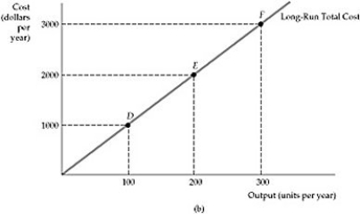 Figure 7.3.4
-Refer to Figure 7.3.4 above. The long run cost curve comes from:
A) a map of isoquants.
B) a map of isocosts.
C) an expansion path.
D) an optimal combination of inputs for a given level of output.
Correct Answer:

Verified
Correct Answer:
Verified
Q123: Scenario 7.3:<br>Use the production function: Q =
Q124: Assume that a firm spends $500 on
Q125: A cubic cost function implies:<br>A) linear average
Q126: <img src="https://d2lvgg3v3hfg70.cloudfront.net/TB3095/.jpg" alt=" Figure 7.2.1 -Refer
Q127: <img src="https://d2lvgg3v3hfg70.cloudfront.net/TB3095/.jpg" alt=" Figure 7.2.1 -Refer
Q129: From the profit maximizing conditions for the
Q130: The total cost (TC) of producing computer
Q131: Consider the following statements when answering this
Q132: Suppose our firm produces chartered business flights
Q133: Scenario 7.3:<br>Use the production function: Q =