TABLE 15- 8
the Superintendent of a School District Wanted

Short Answer

TABLE 15- 8
The superintendent of a school district wanted to predict the percentage of students passing a sixth- grade proficiency test. She obtained the data on percentage of students passing the proficiency test (% Passing), daily average of the percentage of students attending class (% Attendance), average teacher salary in dollars (Salaries), and instructional spending per pupil in dollars (Spending) of 47 schools in the state.
Let Y = % Passing as the dependent variable, X₁ = % Attendance, X₂ = Salaries and X₃ = Spending.
The coefficient of multiple determination (R ² _j) of each of the 3 predictors with all the other remaining predictors are,

respectively, 0.0338, 0.4669, and 0.4743.
The output from the best- subset regressions is given below:
$\begin{array}{llcclcc} & & & && \text {Adjusted} \\\text {Model }&\text { Variables} & \mathrm{Cp} & \mathrm{k} &\text {R Square} & \text {R Square} & \text {Std. Error }\\\hline 1 & X1 & 3.05 & 2 & 0.6024 & 0.5936 & 10.5787 \\2 & X1X2 & 3.66 & 3 & 0.6145 & 0.5970 & 10.5350 \\3 & X1X2X3 & 4.00 & 4 & 0.6288 & 0.6029 & 10.4570 \\4 & X1X3 & 2.00 & 3 & 0.6288 & 0.6119 & 10.3375 \\5 & X2 & 67.35 & 2 & 0.0474 & 0.0262 & 16.3755 \\6 & X2X3 & 64.30 & 3 & 0.0910 & 0.0497 & 16.1768 \\7 & X3 & 62.33 & 2 & 0.0907 & 0.0705 & 15.9984 \\\hline\end{array}$

Following is the residual plot for % Attendance: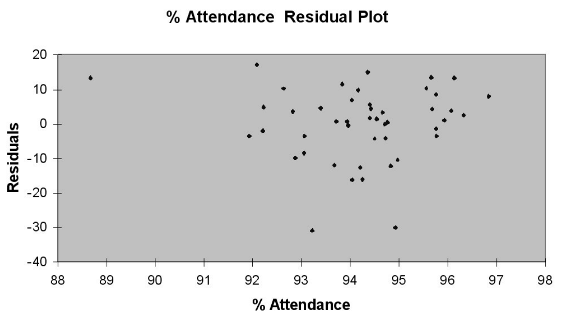



Following is the output of several multiple regression models:

$\text {Model (I):}$
$\begin{array}{lcrclcr}\hline & \text {Coefficients }& \text {Std Error} & \text {Stat } & \text {p-value} & \text { Lower 95\% }& \text { Upper 95\%} \\\hline \text { Intercept} & -753.4225 & 101.1149 & -7.4511 & 2.88 \mathrm{E}-09 & -957.3401 & -549.5050 \\\% \text {Attend }& 8.5014 & 1.0771 & 7.8929 &6.73 \mathrm{E}-10 & 6.3292 & 10.6735 \\ \text {Salary }& 6.85 \mathrm{E}-07 & 0.0006 & 0.0011 & 0.9991 & -0.0013 & 0.0013 \\ \text {Spending} & 0.0060 & 0.0046 & 1.2879 & 0.2047 & -0.0034 & 0.0153 \\\hline\end{array}$


$\text {Model (II):}$
$\begin{array}{lcccc}\hline & \text {Coefficients} & \text {Standard Error }& \text { t Stat} & \text { p -value } \\\hline \text {Intercept }& -753.4086 & 99.1451 & -7.5991 & 1.5291 \mathrm{E}-09 \\\% \text {Attendance} & 8.5014 & 1.0645 & 7.9862 & 4.223 \mathrm{E}-10 \\ \text {Spending} & 0.0060 & 0.0034 & 1.7676 & 0.0840 \\\hline\end{array}$


$\text {Model (III):}$
$\begin{array}{lrrrrl}\hline & \text { d f } & \text { SS } & \text { MS } & \text { F } & \text { Significance F } \\\hline \text { Regression} & 2 & 8162.9429 & 4081.4714 & 39.8708 &1.3201 \mathrm{E}-10 \\ \text { Residual} & 44 & 4504.1635 & 102.3674 & & \\ \text { Total} & 46 & 12667.1064 & & & \\\hline\end{array}$


$\begin{array}{lrcrr}\hline & \text {Coefficients }& \text {Standard Error} & \text { t Stat }& \text {p -value} \\\hline \text {Intercept }& 6672.8367 & 3267.7349 & 2.0420 & 0.0472 \\\% \text { Attendance} & -150.5694 & 69.9519 & -2.1525 & 0.0369 \\\% \text {Attendance Squared}& 0.8532 & 0.3743 & 2.2792 & 0.0276 \\\hline\end{array}$




-Referring to Table 15-8, what is the p-value of the test statistic to determine whether the quadratic effect of daily average of the percentage of students attending class on percentage of students passing the proficiency test is significant at a 5% level of significance?