Deck 13: Simple Linear Regression
Full screen (f)
Question
Question
Question
Question
Question
TABLE 13-12
The manager of the purchasing department of a large banking organization would like to develop a model to predict the amount of time (measured in hours) it takes to process invoices. Data are collected from a sample of 30 days, and the number of invoices processed and completion time in hours is recorded. Below is the regression output:

-Referring to Table 13-12, the degrees of freedom for the F test on whether the number of invoices processed affects the amount of time are
A) 1, 29.
B) 28, 1.
C) 29, 1.
D) 1, 28.
The manager of the purchasing department of a large banking organization would like to develop a model to predict the amount of time (measured in hours) it takes to process invoices. Data are collected from a sample of 30 days, and the number of invoices processed and completion time in hours is recorded. Below is the regression output:
-Referring to Table 13-12, the degrees of freedom for the F test on whether the number of invoices processed affects the amount of time are
A) 1, 29.
B) 28, 1.
C) 29, 1.
D) 1, 28.
Question
Question
TABLE 13-9
It is believed that, the average numbers of hours spent studying per day (HOURS) during undergraduate education should have a positive linear relationship with the starting salary (SALARY, measured in thousands of dollars per month) after graduation. Given below is the Excel output from regressing starting salary on number of hours spent studying per day for a sample of 51 students. NOTE: Some of the numbers in the output are purposely erased.
![<strong>TABLE 13-9 It is believed that, the average numbers of hours spent studying per day (HOURS) during undergraduate education should have a positive linear relationship with the starting salary (SALARY, measured in thousands of dollars per month) after graduation. Given below is the Excel output from regressing starting salary on number of hours spent studying per day for a sample of 51 students. NOTE: Some of the numbers in the output are purposely erased. \begin{array}{l} \text { Regression Statistics }\\ \begin{array} { l c } \hline \text { Multiple R } & 0.8857 \\ \text { R Square } & 0.7845 \\ \text { Adjusted R Square } & 0.7801 \\ \text { Standard Error } & 1.3704 \\ \text { Observations } & 51 \\ \hline \end{array} \end{array} \text { ANOVA } \begin{array}{llcc} \hline&\text { df }&\text { SS } &\text { MS }&\text {F }&\text { Significance F } \\ \text { Regression } & 1 & 335.0472 & 335.0473 & 178.3859 \\ \text { Residual } & & & 1.8782 & \\ \text { Total } & 50 & 427.0798 & & \end{array} -Referring to Table 13-9, the 90% confidence interval for the average change in SALARY (in thousands of dollars) as a result of spending an extra hour per day studying is</strong> A) wider than [-2.70159, -1.08654]. B) wider than [0.8321927, 1.12697]. C) narrower than [0.8321927, 1.12697]. D) narrower than [-2.70159, -1.08654]. <div style=padding-top: 35px>](https://storage.examlex.com/TB1603/11eae851_7ada_b58c_8aff_8f2635bff296_TB1603_00.jpg)
-Referring to Table 13-9, the 90% confidence interval for the average change in SALARY (in thousands of dollars) as a result of spending an extra hour per day studying is
A) wider than [-2.70159, -1.08654].
B) wider than [0.8321927, 1.12697].
C) narrower than [0.8321927, 1.12697].
D) narrower than [-2.70159, -1.08654].
It is believed that, the average numbers of hours spent studying per day (HOURS) during undergraduate education should have a positive linear relationship with the starting salary (SALARY, measured in thousands of dollars per month) after graduation. Given below is the Excel output from regressing starting salary on number of hours spent studying per day for a sample of 51 students. NOTE: Some of the numbers in the output are purposely erased.
-Referring to Table 13-9, the 90% confidence interval for the average change in SALARY (in thousands of dollars) as a result of spending an extra hour per day studying is
A) wider than [-2.70159, -1.08654].
B) wider than [0.8321927, 1.12697].
C) narrower than [0.8321927, 1.12697].
D) narrower than [-2.70159, -1.08654].
Question
Question
Question
Question
Question
Question
Question
TABLE 13-9
It is believed that, the average numbers of hours spent studying per day (HOURS) during undergraduate education should have a positive linear relationship with the starting salary (SALARY, measured in thousands of dollars per month) after graduation. Given below is the Excel output from regressing starting salary on number of hours spent studying per day for a sample of 51 students. NOTE: Some of the numbers in the output are purposely erased.

-Referring to Table 13-9, the estimated average change in salary (in thousands of dollars) as a result of spending an extra hour per day studying is
A) 0.9795.
B) -1.8940.
C) 0.7845.
D) 335.0473.
It is believed that, the average numbers of hours spent studying per day (HOURS) during undergraduate education should have a positive linear relationship with the starting salary (SALARY, measured in thousands of dollars per month) after graduation. Given below is the Excel output from regressing starting salary on number of hours spent studying per day for a sample of 51 students. NOTE: Some of the numbers in the output are purposely erased.
-Referring to Table 13-9, the estimated average change in salary (in thousands of dollars) as a result of spending an extra hour per day studying is
A) 0.9795.
B) -1.8940.
C) 0.7845.
D) 335.0473.
Question
TABLE 13-12
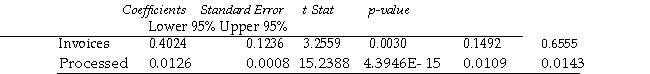
The manager of the purchasing department of a large banking organization would like to develop a model to predict the amount of time (measured in hours) it takes to process invoices. Data are collected from a sample of 30 days, and the number of invoices processed and completion time in hours is recorded. Below is the regression output:
![<strong>TABLE 13-12 The manager of the purchasing department of a large banking organization would like to develop a model to predict the amount of time (measured in hours) it takes to process invoices. Data are collected from a sample of 30 days, and the number of invoices processed and completion time in hours is recorded. Below is the regression output: \begin{array} { l c } { \text { Regression } \text { Statistics } } \\ \hline \text { Multiple R } & 0.9947 \\ \text { R Square } & 0.8924 \\ \text { Adjusted R Square } & 0.8886 \\ \text { Standard Error } & 0.3342 \\ \text { Observations } & 30 \\ \hline \end{array} \begin{array}{l} \text { ANOVA }\\ \begin{array} { l c c c c c } & d f & \text { SS } & \text { MS } & F & \text { Significance } F \\ \text { Regression } & 1 & 25.9438&25 .9438 & 232.2200&4 .3946 \mathrm { E } - 15 \\ \text { Residual } & 28 & 3.12820 .1117 & \\ \text { Total } & 29 & 29.072 \\ \hline \end{array} \end{array} \begin{array} { l r r r r r r } \hline & \text { Coefficients } & \text { Standard Enror } & t \text { Stat } & p \text {-value } & \text { Lower 95\% } & \text { Upper 95\% } \\ \hline \text { Invoices } & 0.4024 & 0.1236 & 3.2559 & 0.0030 & 0.1492 & 0.6555 \\ \text { Processed } & 0.0126 & 0.0008 & 15.2388 & 4.3946 \mathrm { E } 15 & 0.0109 & 0.0143 \end{array} \begin{array}{rrrrrrr} & \text { Coefficients } & \text { Standard Enor } & \text { t Stat } & p \text {-value } & \text { Lower 95\% } & \text { Upper 95\% } \\ \hline \text { Invoices } & 0.4024 & 0.1236 & 3.2559 & 0.0030 & 0.1492 & 0.6555 \end{array} -Referring to Table 13-12, the 90% confidence interval for the average change in the amount of time needed as a result of processing one additional invoice is</strong> A) narrower than [0.0109, 0.0143]. B) wider than [0.0109, 0.0143]. C) narrower than [0.1492, 0.6555]. D) wider than [0.1492, 0.6555]. <div style=padding-top: 35px>](https://storage.examlex.com/TB1603/11eae851_7ada_4054_8aff_856ca452bc33_TB1603_00.jpg)
![<strong>TABLE 13-12 The manager of the purchasing department of a large banking organization would like to develop a model to predict the amount of time (measured in hours) it takes to process invoices. Data are collected from a sample of 30 days, and the number of invoices processed and completion time in hours is recorded. Below is the regression output: \begin{array} { l c } { \text { Regression } \text { Statistics } } \\ \hline \text { Multiple R } & 0.9947 \\ \text { R Square } & 0.8924 \\ \text { Adjusted R Square } & 0.8886 \\ \text { Standard Error } & 0.3342 \\ \text { Observations } & 30 \\ \hline \end{array} \begin{array}{l} \text { ANOVA }\\ \begin{array} { l c c c c c } & d f & \text { SS } & \text { MS } & F & \text { Significance } F \\ \text { Regression } & 1 & 25.9438&25 .9438 & 232.2200&4 .3946 \mathrm { E } - 15 \\ \text { Residual } & 28 & 3.12820 .1117 & \\ \text { Total } & 29 & 29.072 \\ \hline \end{array} \end{array} \begin{array} { l r r r r r r } \hline & \text { Coefficients } & \text { Standard Enror } & t \text { Stat } & p \text {-value } & \text { Lower 95\% } & \text { Upper 95\% } \\ \hline \text { Invoices } & 0.4024 & 0.1236 & 3.2559 & 0.0030 & 0.1492 & 0.6555 \\ \text { Processed } & 0.0126 & 0.0008 & 15.2388 & 4.3946 \mathrm { E } 15 & 0.0109 & 0.0143 \end{array} \begin{array}{rrrrrrr} & \text { Coefficients } & \text { Standard Enor } & \text { t Stat } & p \text {-value } & \text { Lower 95\% } & \text { Upper 95\% } \\ \hline \text { Invoices } & 0.4024 & 0.1236 & 3.2559 & 0.0030 & 0.1492 & 0.6555 \end{array} -Referring to Table 13-12, the 90% confidence interval for the average change in the amount of time needed as a result of processing one additional invoice is</strong> A) narrower than [0.0109, 0.0143]. B) wider than [0.0109, 0.0143]. C) narrower than [0.1492, 0.6555]. D) wider than [0.1492, 0.6555]. <div style=padding-top: 35px>](https://storage.examlex.com/TB1603/11eae851_7ada_4055_8aff_3f5e5b9e05d2_TB1603_00.jpg)
-Referring to Table 13-12, the 90% confidence interval for the average change in the amount of time needed as a result of processing one additional invoice is
A) narrower than [0.0109, 0.0143].
B) wider than [0.0109, 0.0143].
C) narrower than [0.1492, 0.6555].
D) wider than [0.1492, 0.6555].
The manager of the purchasing department of a large banking organization would like to develop a model to predict the amount of time (measured in hours) it takes to process invoices. Data are collected from a sample of 30 days, and the number of invoices processed and completion time in hours is recorded. Below is the regression output:
-Referring to Table 13-12, the 90% confidence interval for the average change in the amount of time needed as a result of processing one additional invoice is
A) narrower than [0.0109, 0.0143].
B) wider than [0.0109, 0.0143].
C) narrower than [0.1492, 0.6555].
D) wider than [0.1492, 0.6555].
Question
Question
Question
Question
TABLE 13-12
The manager of the purchasing department of a large banking organization would like to develop a model to predict the amount of time (measured in hours) it takes to process invoices. Data are collected from a sample of 30 days, and the number of invoices processed and completion time in hours is recorded. Below is the regression output:

-Referring to Table 13-12, the degrees of freedom for the t test on whether the number of invoices processed affects the amount of time are
A) 1.
B) 28.
C) 30.
D) 29.
The manager of the purchasing department of a large banking organization would like to develop a model to predict the amount of time (measured in hours) it takes to process invoices. Data are collected from a sample of 30 days, and the number of invoices processed and completion time in hours is recorded. Below is the regression output:
-Referring to Table 13-12, the degrees of freedom for the t test on whether the number of invoices processed affects the amount of time are
A) 1.
B) 28.
C) 30.
D) 29.
Question
Question
Question
Question
Question
Question
TABLE 13-12
The manager of the purchasing department of a large banking organization would like to develop a model to predict the amount of time (measured in hours) it takes to process invoices. Data are collected from a sample of 30 days, and the number of invoices processed and completion time in hours is recorded. Below is the regression output:
-Referring to Table 13-12, the p-value of the measured t-test statistic to test whether the number of invoices processed affects the amount of time is
A) (0.0030)/2.
B) 0.0030.
C) 4.3946E-15.
D) (4.3946E-15)/2.
Question
Question
Question
Question
Question
TABLE 13- 11
A company that has the distribution rights to home video sales of previously released movies would like to use the box office gross (in millions of dollars) to estimate the number of units (in thousands of units) that it can expect to sell. Following is the output from a simple linear regression along with the residual plot and normal probability plot obtained from a data set of 30 different movie titles:
ANOVA
-Referring to Table 13-11, which of the following is the correct interpretation for the slope coefficient?
A) For each increase of 1 dollar in box office gross, expected home video units sold are estimated to increase by 4.3331 thousand units.
B) For each increase of 1 million dollars in box office gross, expected home video units sold are estimated to increase by 4.3331 units.
C) For each increase of 1 dollar in box office gross, expected home video units sold are estimated to increase by 4.3331 units.
D) For each increase of 1 million dollars in box office gross, expected home video units sold are estimated to increase by 4.3331 thousand units.
Question
Question
Question
Question
Question
Question
Question
Question
Question
Question
Question
Question
Question
Question
Question
Question
Question
Question
Question
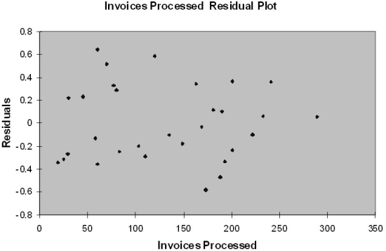
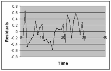
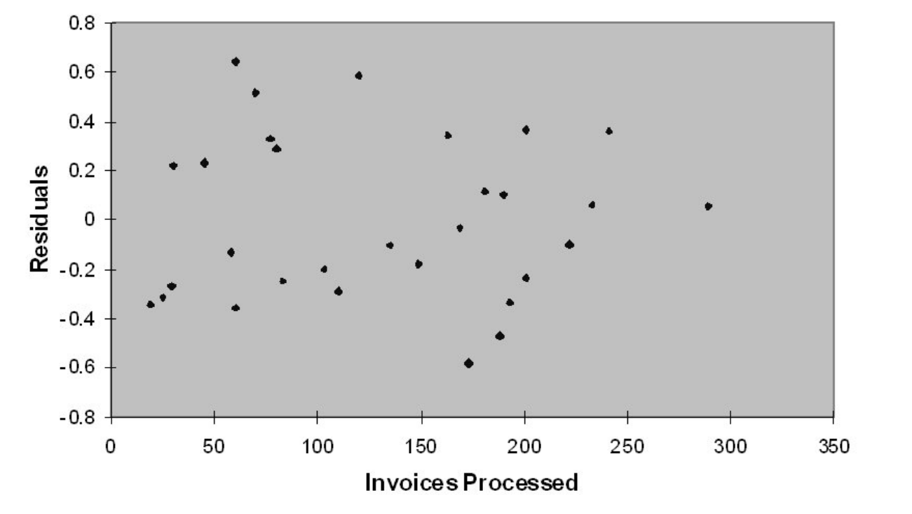
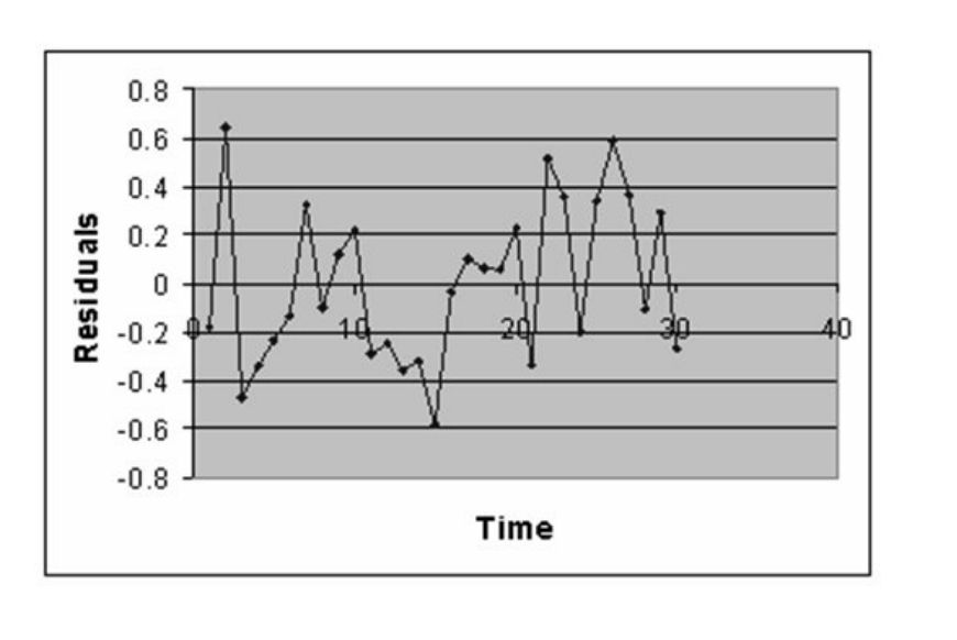
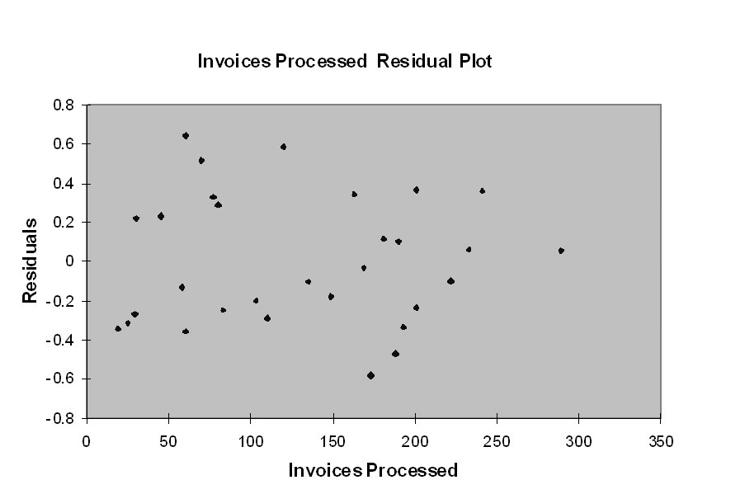
Based on the residual plot below, you will conclude that there might be a violation of which of the following assumptions?
A) Homoscedasticity
B) Independence of errors
C) Normality of errors
D) Linearity of the relationship
A) Homoscedasticity
B) Independence of errors
C) Normality of errors
D) Linearity of the relationship
Question
TABLE 13-12
The manager of the purchasing department of a large banking organization would like to develop a model to predict the amount of time (measured in hours) it takes to process invoices. Data are collected from a sample of 30 days, and the number of invoices processed and completion time in hours is recorded. Below is the regression output:
-Referring to Table 13-12, the p-value of the measured F-test statistic to test whether the number of invoices processed affects the amount of time is
A) (4.3946E-15)/2.
B) (0.0030)/2.
C) 0.0030.
D) 4.3946E-15.
Question
Question
TABLE 13- 11
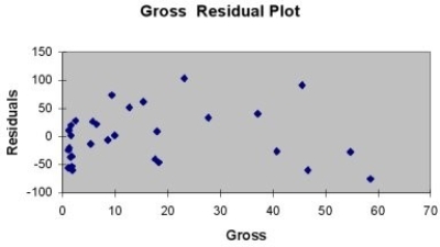
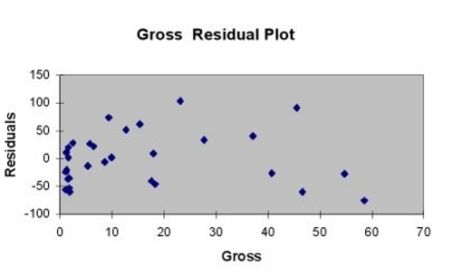
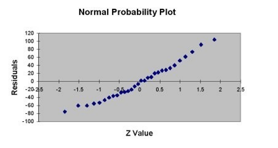
A company that has the distribution rights to home video sales of previously released movies would like to use the box office gross (in millions of dollars) to estimate the number of units (in thousands of units) that it can expect to sell. Following is the output from a simple linear regression along with the residual plot and normal probability plot obtained from a data set of 30 different movie titles:
ANOVA
-Referring to Table 13-11, which of the following assumptions appears to have been violated?
A) homoscedasticity
B) independence of errors
C) normality of error
D) none of the above
Question
Question
Question
TABLE 13-12
The manager of the purchasing department of a large banking organization would like to develop a model to predict the amount of time (measured in hours) it takes to process invoices. Data are collected from a sample of 30 days, and the number of invoices processed and completion time in hours is recorded. Below is the regression output:
-Referring to Table 13-12, the error sum of squares (SSE) of the above regression is
A) 0.1117.
B) 29.0720.
C) 25.9438.
D) 3.1282.
Question
Question
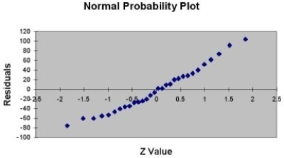
TABLE 13- 11
A company that has the distribution rights to home video sales of previously released movies would like to use the box office gross (in millions of dollars) to estimate the number of units (in thousands of units) that it can expect to sell. Following is the output from a simple linear regression along with the residual plot and normal probability plot obtained from a data set of 30 different movie titles:
ANOVA
-Referring to Table 13-11, which of the following is the correct alternative hypothesis for testing whether there is a linear relationship between box office gross and home video unit sales?
A)
B)
C)
D)
Question
Question
Question
Question
Question
Question
Question
Question
Question
Question
TABLE 13-12
The manager of the purchasing department of a large banking organization would like to develop a model to predict the amount of time (measured in hours) it takes to process invoices. Data are collected from a sample of 30 days, and the number of invoices processed and completion time in hours is recorded. Below is the regression output:
-Referring to Table 13-12, the estimated average amount of time it takes to process one additional invoice is
A) 0.0126 more hours.
B) 0.0126 fewer hours.
C) 0.4024 more hours.
D) 0.4024 fewer hours.
Question
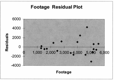
TABLE 13- 11
A company that has the distribution rights to home video sales of previously released movies would like to use the box office gross (in millions of dollars) to estimate the number of units (in thousands of units) that it can expect to sell. Following is the output from a simple linear regression along with the residual plot and normal probability plot obtained from a data set of 30 different movie titles:
ANOVA
-Referring to Table 13-11, what is the standard deviation around the regression line?
Question
Question
Question
Question
Question
TABLE 13- 11
A company that has the distribution rights to home video sales of previously released movies would like to use the box office gross (in millions of dollars) to estimate the number of units (in thousands of units) that it can expect to sell. Following is the output from a simple linear regression along with the residual plot and normal probability plot obtained from a data set of 30 different movie titles:
ANOVA
-Referring to Table 13-11, which of the following is the correct interpretation for the coefficient of determination?
A) 72.8% of the variation in the box office gross can be explained by the variation in the video unit sales.
B) 71.8% of the variation in the video unit sales can be explained by the variation in the box office gross.
C) 71.8% of the variation in the box office gross can be explained by the variation in the video unit sales.
D) 72.8% of the variation in the video unit sales can be explained by the variation in the box office gross.
Question
Question
Question
TABLE 13-12
The manager of the purchasing department of a large banking organization would like to develop a model to predict the amount of time (measured in hours) it takes to process invoices. Data are collected from a sample of 30 days, and the number of invoices processed and completion time in hours is recorded. Below is the regression output:
-Referring to Table 13-12, the value of the measured t-test statistic to test whether the amount of time depends linearly on the number of invoices processed is
A) 0.8924.
B) 15.2388.
C) 232.2200.
D) 3.2559.
Question
Question
Question
Question

Unlock Deck
Sign up to unlock the cards in this deck!
Unlock Deck
Unlock Deck
1/196
Play
Full screen (f)
Deck 13: Simple Linear Regression
1
TABLE 13-10
The management of a chain electronic store would like to develop a model for predicting the weekly sales (in thousand of dollars) for individual stores based on the number of customers who made purchases. A random sample of 12 stores yields the following results:
-Referring to Table 13-10, which is the correct null hypothesis for testing whether the number of customers who make purchase affects weekly sales?
A) H0 : ?0 = 0
B) H0 : µ = 0
C) H0 : ?1 = 0
D) H0 : ?= 0
H0 : ?1 = 0
2
TABLE 13-7
An investment specialist claims that if one holds a portfolio that moves in the opposite direction to the market index like the S&P 500, then it is possible to reduce the variability of the portfolio's return. In other words, one can create a portfolio with positive returns but less exposure to risk. A sample of 26 years of S&P 500 index and a portfolio consisting of stocks of private prisons, which are believed to be negatively related to the S&P 500 index, is collected. A regression analysis was performed by regressing the returns of the prison stocks portfolio (Y) on the returns of S&P 500 index (X) to prove that the prison stocks portfolio is negatively related to the S&P 500 index at a 5% level of significance. The results are given in the following EXCEL output.
-Referring to Table 13-7, to test whether the prison stocks portfolio is negatively related to the S&P 500 index, the measured value of the test statistic is
A) 0.357.
B) 0.072.
C) -0.503.
D) -7.019.
-7.019.
3
TABLE 13-2
A candy bar manufacturer is interested in trying to estimate how sales are influenced by the price of their product. To do this, the company randomly chooses 6 small cities and offers the candy bar at different prices. Using candy bar sales as the dependent variable, the company will conduct a simple linear regression on the data below:
-Referring to Table 13-2, what is for these data?
A) 2.54
B) 0
C) 1.66
D) 25.66
1.66
4
TABLE 13-2
A candy bar manufacturer is interested in trying to estimate how sales are influenced by the price of their product. To do this, the company randomly chooses 6 small cities and offers the candy bar at different prices. Using candy bar sales as the dependent variable, the company will conduct a simple linear regression on the data below:
-Referring to Table 13-2, what is the coefficient of correlation for these data?
A) - 0.7839
B) 0.8854
C) 0.7839
D) - 0.8854
Unlock Deck
Unlock for access to all 196 flashcards in this deck.
Unlock Deck
k this deck
5
TABLE 13-12
The manager of the purchasing department of a large banking organization would like to develop a model to predict the amount of time (measured in hours) it takes to process invoices. Data are collected from a sample of 30 days, and the number of invoices processed and completion time in hours is recorded. Below is the regression output:
-Referring to Table 13-12, the degrees of freedom for the F test on whether the number of invoices processed affects the amount of time are
A) 1, 29.
B) 28, 1.
C) 29, 1.
D) 1, 28.
Unlock Deck
Unlock for access to all 196 flashcards in this deck.
Unlock Deck
k this deck
6
TABLE 13-2
A candy bar manufacturer is interested in trying to estimate how sales are influenced by the price of their product. To do this, the company randomly chooses 6 small cities and offers the candy bar at different prices. Using candy bar sales as the dependent variable, the company will conduct a simple linear regression on the data below:
-The sample correlation coefficient between X and Y is 0.375. It has been found out that the p- value is 0.744 when testing H0 : ? = 0 against the one- sided alternative H0 : ? < 0. To test H0 : ? = 0 against the two- sided alternative H0 : ?? 0 at a significance level of 0.2, the p- value is
A) (1 - 0.744)(2).
B) (0.744)(2).
C) 0.744/2.
D) 1 - 0.744.
Unlock Deck
Unlock for access to all 196 flashcards in this deck.
Unlock Deck
k this deck
7
TABLE 13-9
It is believed that, the average numbers of hours spent studying per day (HOURS) during undergraduate education should have a positive linear relationship with the starting salary (SALARY, measured in thousands of dollars per month) after graduation. Given below is the Excel output from regressing starting salary on number of hours spent studying per day for a sample of 51 students. NOTE: Some of the numbers in the output are purposely erased.
-Referring to Table 13-9, the 90% confidence interval for the average change in SALARY (in thousands of dollars) as a result of spending an extra hour per day studying is
A) wider than [-2.70159, -1.08654].
B) wider than [0.8321927, 1.12697].
C) narrower than [0.8321927, 1.12697].
D) narrower than [-2.70159, -1.08654].
Unlock Deck
Unlock for access to all 196 flashcards in this deck.
Unlock Deck
k this deck
8
Which of the following assumptions concerning the probability distribution of the random error term is stated incorrectly?
A) The variance of the distribution increases as X increases.
B) The distribution is normal.
C) The errors are independent.
D) The mean of the distribution is 0.
A) The variance of the distribution increases as X increases.
B) The distribution is normal.
C) The errors are independent.
D) The mean of the distribution is 0.
Unlock Deck
Unlock for access to all 196 flashcards in this deck.
Unlock Deck
k this deck
9
TABLE 13-9
It is believed that, the average numbers of hours spent studying per day (HOURS) during undergraduate education should have a positive linear relationship with the starting salary (SALARY, measured in thousands of dollars per month) after graduation. Given below is the Excel output from regressing starting salary on number of hours spent studying per day for a sample of 51 students. NOTE: Some of the numbers in the output are purposely erased.
-Referring to Table 13-9, the value of the measured t-test statistic to test whether average SALARY depends linearly on HOURS is
A) 13.3561.
B) 0.9795.
C) -4.7134.
D) -1.8940.
Unlock Deck
Unlock for access to all 196 flashcards in this deck.
Unlock Deck
k this deck
10
TABLE 13-2
A candy bar manufacturer is interested in trying to estimate how sales are influenced by the price of their product. To do this, the company randomly chooses 6 small cities and offers the candy bar at different prices. Using candy bar sales as the dependent variable, the company will conduct a simple linear regression on the data below:
-Referring to Table 13-2, what is the percentage of the total variation in candy bar sales explained by the regression model?
A) 78.39%
B) 100%
C) 48.19%
D) 88.54%
Unlock Deck
Unlock for access to all 196 flashcards in this deck.
Unlock Deck
k this deck
11
TABLE 13-9
It is believed that, the average numbers of hours spent studying per day (HOURS) during undergraduate education should have a positive linear relationship with the starting salary (SALARY, measured in thousands of dollars per month) after graduation. Given below is the Excel output from regressing starting salary on number of hours spent studying per day for a sample of 51 students. NOTE: Some of the numbers in the output are purposely erased.
-Referring to Table 13-9, the degrees of freedom for the F test on whether HOURS affects SALARY are
A) 50, 1.
B) 1, 50.
C) 49, 1.
D) 1, 49.
Unlock Deck
Unlock for access to all 196 flashcards in this deck.
Unlock Deck
k this deck
12
If you wanted to find out if alcohol consumption (measured in fluid oz.) and grade point average on a 4-point scale are linearly related, you would perform a
A) a t test for a correlation coefficient.
B) ?2 test for independence.
C) ?2 test for the difference in two proportions.
D) a Z test for the difference in two proportions.
A) a t test for a correlation coefficient.
B) ?2 test for independence.
C) ?2 test for the difference in two proportions.
D) a Z test for the difference in two proportions.
Unlock Deck
Unlock for access to all 196 flashcards in this deck.
Unlock Deck
k this deck
13
Testing for the existence of correlation is equivalent to
A) the confidence interval estimate for predicting Y.
B) testing for the existence of the slope (?1).
C) testing for the existence of the Y-intercept (?2).
D) none of the above
A) the confidence interval estimate for predicting Y.
B) testing for the existence of the slope (?1).
C) testing for the existence of the Y-intercept (?2).
D) none of the above
Unlock Deck
Unlock for access to all 196 flashcards in this deck.
Unlock Deck
k this deck
14
TABLE 13-9
It is believed that, the average numbers of hours spent studying per day (HOURS) during undergraduate education should have a positive linear relationship with the starting salary (SALARY, measured in thousands of dollars per month) after graduation. Given below is the Excel output from regressing starting salary on number of hours spent studying per day for a sample of 51 students. NOTE: Some of the numbers in the output are purposely erased.
-Referring to Table 13-9, the estimated average change in salary (in thousands of dollars) as a result of spending an extra hour per day studying is
A) 0.9795.
B) -1.8940.
C) 0.7845.
D) 335.0473.
Unlock Deck
Unlock for access to all 196 flashcards in this deck.
Unlock Deck
k this deck
15
TABLE 13-12
The manager of the purchasing department of a large banking organization would like to develop a model to predict the amount of time (measured in hours) it takes to process invoices. Data are collected from a sample of 30 days, and the number of invoices processed and completion time in hours is recorded. Below is the regression output:
-Referring to Table 13-12, the 90% confidence interval for the average change in the amount of time needed as a result of processing one additional invoice is
A) narrower than [0.0109, 0.0143].
B) wider than [0.0109, 0.0143].
C) narrower than [0.1492, 0.6555].
D) wider than [0.1492, 0.6555].
Unlock Deck
Unlock for access to all 196 flashcards in this deck.
Unlock Deck
k this deck
16
TABLE 13-2
A candy bar manufacturer is interested in trying to estimate how sales are influenced by the price of their product. To do this, the company randomly chooses 6 small cities and offers the candy bar at different prices. Using candy bar sales as the dependent variable, the company will conduct a simple linear regression on the data below:
-Referring to Table 13-2, if the price of the candy bar is set at $2, the estimated average sales will be
A) 30.
B) 90.
C) 100.
D) 65.
Unlock Deck
Unlock for access to all 196 flashcards in this deck.
Unlock Deck
k this deck
17
What do we mean when we say that a simple linear regression model is "statistically" useful?
A) The model is an excellent predictor of Y.
B) The model is a better predictor of Y than the sample mean, Y.
C) The model is "practically" useful for predicting Y.
D) All the statistics computed from the sample make sense.
A) The model is an excellent predictor of Y.
B) The model is a better predictor of Y than the sample mean, Y.
C) The model is "practically" useful for predicting Y.
D) All the statistics computed from the sample make sense.
Unlock Deck
Unlock for access to all 196 flashcards in this deck.
Unlock Deck
k this deck
18
The sample correlation coefficient between X and Y is 0.375. It has been found out that the p- value is 0.256 when testing H0 : q = 0 against the one- sided alternative H0 : q > 0. To test H0 : q = 0 against the two- sided alternative H0 : q × 0 at a significance level of 0.2, the p- value is
A) (0.256)(2).
B) 1 - 0.256/2.
C) 0.256/2.
D) 1 - 0.256.
A) (0.256)(2).
B) 1 - 0.256/2.
C) 0.256/2.
D) 1 - 0.256.
Unlock Deck
Unlock for access to all 196 flashcards in this deck.
Unlock Deck
k this deck
19
TABLE 13-12
The manager of the purchasing department of a large banking organization would like to develop a model to predict the amount of time (measured in hours) it takes to process invoices. Data are collected from a sample of 30 days, and the number of invoices processed and completion time in hours is recorded. Below is the regression output:
-Referring to Table 13-12, the degrees of freedom for the t test on whether the number of invoices processed affects the amount of time are
A) 1.
B) 28.
C) 30.
D) 29.
Unlock Deck
Unlock for access to all 196 flashcards in this deck.
Unlock Deck
k this deck
20
The least squares method minimizes which of the following?
A) SSR
B) SST
C) SSE
D) all of the above
A) SSR
B) SST
C) SSE
D) all of the above
Unlock Deck
Unlock for access to all 196 flashcards in this deck.
Unlock Deck
k this deck
21
TABLE 13-5
The managing partner of an advertising agency believes that his company's sales are related to the industry sales. He uses Microsoft Excel's Data Analysis tool to analyze the last 4 years of quarterly data with the following results:
Durbin- Watson Statistic 1.59
-Referring to Table 13-5, the partner wants to test for autocorrelation using the Durbin-Watson statistic. Using a level of significance of 0.05, the decision he should make is
A) there is no evidence of autocorrelation.
B) there is not enough information to perform the test.
C) there is evidence of autocorrelation.
D) the test is unable to make a definite conclusion.
Unlock Deck
Unlock for access to all 196 flashcards in this deck.
Unlock Deck
k this deck
22
TABLE 13-2
A candy bar manufacturer is interested in trying to estimate how sales are influenced by the price of their product. To do this, the company randomly chooses 6 small cities and offers the candy bar at different prices. Using candy bar sales as the dependent variable, the company will conduct a simple linear regression on the data below:
-Referring to Table 13-2, to test whether a change in price will have any impact on average sales, what would be the critical values? Use ? = 0.05.
A) ±2.7765
B) ±2.5706
C) ±3.1634
D) ±3.4954
Unlock Deck
Unlock for access to all 196 flashcards in this deck.
Unlock Deck
k this deck
23
If the correlation coefficient (r) = 1.00, then
A) there is no explained variation.
B) there is no unexplained variation.
C) the Y-intercept (b0) must equal 0.
D) the explained variation equals the unexplained variation.
A) there is no explained variation.
B) there is no unexplained variation.
C) the Y-intercept (b0) must equal 0.
D) the explained variation equals the unexplained variation.
Unlock Deck
Unlock for access to all 196 flashcards in this deck.
Unlock Deck
k this deck
24
If the plot of the residuals is fan shaped, which assumption is violated?
A) independence of errors
B) normality
C) homoscedasticity
D) No assumptions are violated; the graph should resemble a fan.
A) independence of errors
B) normality
C) homoscedasticity
D) No assumptions are violated; the graph should resemble a fan.
Unlock Deck
Unlock for access to all 196 flashcards in this deck.
Unlock Deck
k this deck
25
TABLE 13-12
The manager of the purchasing department of a large banking organization would like to develop a model to predict the amount of time (measured in hours) it takes to process invoices. Data are collected from a sample of 30 days, and the number of invoices processed and completion time in hours is recorded. Below is the regression output:
-Referring to Table 13-12, the p-value of the measured t-test statistic to test whether the number of invoices processed affects the amount of time is
A) (0.0030)/2.
B) 0.0030.
C) 4.3946E-15.
D) (4.3946E-15)/2.
Unlock Deck
Unlock for access to all 196 flashcards in this deck.
Unlock Deck
k this deck
26
Assuming a linear relationship between X and Y, if the coefficient of correlation (r) equals - 0.30,
A) the slope (b1) is negative.
B) there is no correlation.
C) variable X is larger than variable Y.
D) the variance of X is negative.
A) the slope (b1) is negative.
B) there is no correlation.
C) variable X is larger than variable Y.
D) the variance of X is negative.
Unlock Deck
Unlock for access to all 196 flashcards in this deck.
Unlock Deck
k this deck
27
TABLE 13-01
A large national bank charges local companies for using their services. A bank official reported the results of a regression analysis designed to predict the bank's charges (Y) -- measured in dollars per month -- for services rendered to local companies. One independent variable used to predict service charge to a company is the company's sales revenue (X) -- measured in millions of dollars. Data for 21 companies who use the bank's services were used to fit the model:
The results of the simple linear regression are provided below.
-Referring to Table 13-1, interpret the p-value for testing whether þ1 exceeds 0.
A) There is sufficient evidence (at the ? = 0.05) to conclude that sales revenue (X) is a useful linear predictor of service charge (Y).
B) For every $1 million increase in sales revenue, we expect a service charge to increase $0.034.
C) There is insufficient evidence (at the ? = 0.10) to conclude that sales revenue (X) is a useful linear predictor of service charge (Y).
D) Sales revenue (X) is a poor predictor of service charge (Y).
Unlock Deck
Unlock for access to all 196 flashcards in this deck.
Unlock Deck
k this deck
28
TABLE 13-2
A candy bar manufacturer is interested in trying to estimate how sales are influenced by the price of their product. To do this, the company randomly chooses 6 small cities and offers the candy bar at different prices. Using candy bar sales as the dependent variable, the company will conduct a simple linear regression on the data below:
-Referring to Table 13-2, what percentage of the total variation in candy bar sales is explained by prices?
A) 100%
B) 78.39%
C) 88.54%
D) 48.19%
Unlock Deck
Unlock for access to all 196 flashcards in this deck.
Unlock Deck
k this deck
29
The Y-intercept (b0) represents the
A) change in estimated average Y per unit change in X.
B) variation around the sample regression line.
C) predicted value of Y.
D) estimated average Y when X = 0.
A) change in estimated average Y per unit change in X.
B) variation around the sample regression line.
C) predicted value of Y.
D) estimated average Y when X = 0.
Unlock Deck
Unlock for access to all 196 flashcards in this deck.
Unlock Deck
k this deck
30
TABLE 13- 11
A company that has the distribution rights to home video sales of previously released movies would like to use the box office gross (in millions of dollars) to estimate the number of units (in thousands of units) that it can expect to sell. Following is the output from a simple linear regression along with the residual plot and normal probability plot obtained from a data set of 30 different movie titles:
ANOVA
-Referring to Table 13-11, which of the following is the correct interpretation for the slope coefficient?
A) For each increase of 1 dollar in box office gross, expected home video units sold are estimated to increase by 4.3331 thousand units.
B) For each increase of 1 million dollars in box office gross, expected home video units sold are estimated to increase by 4.3331 units.
C) For each increase of 1 dollar in box office gross, expected home video units sold are estimated to increase by 4.3331 units.
D) For each increase of 1 million dollars in box office gross, expected home video units sold are estimated to increase by 4.3331 thousand units.
Unlock Deck
Unlock for access to all 196 flashcards in this deck.
Unlock Deck
k this deck
31
TABLE 13-01
A large national bank charges local companies for using their services. A bank official reported the results of a regression analysis designed to predict the bank's charges
The results of the simple linear regression are provided below.
(Y) -- measured in dollars per month -- for services rendered to local companies. One independent variable used to predict service charge to a company is the company's sales revenue (X) -- measured in millions of dollars. Data for 21 companies who use the bank's services were used to fit the model:
-Referring to Table 13-1, interpret the estimate of a, the standard deviation of the random error term (standard error of the estimate) in the model.
A) About 95% of the observed service charges fall within $130 of the least squares line.
B) For every $1 million increase in sales revenue, we expect a service charge to increase $65.
C) About 95% of the observed service charges fall within $65 of the least squares line.
D) About 95% of the observed service charges equal their corresponding predicted values.
Unlock Deck
Unlock for access to all 196 flashcards in this deck.
Unlock Deck
k this deck
32
TABLE 13-01
A large national bank charges local companies for using their services. A bank official reported the results of a regression analysis designed to predict the bank's charges (Y) -- measured in dollars per month -- for services rendered to local companies. One independent variable used to predict service charge to a company is the company's sales revenue (X) -- measured in millions of dollars. Data for 21 companies who use the bank's services were used to fit the model:
E(Y) =?0 + ?1X
The results of the simple linear regression are provided below.
, two-tailed value for testing
-Referring to Table 13-1, a 95% confidence interval for ?1 is (15, 30). Interpret the interval.
A) At the ? = 0.05 level, there is no evidence of a linear relationship between service charge (Y) and sales revenue (X).
B) We are 95% confident that the mean service charge will fall between $15 and $30 per month.
C) We are 95% confident that average service charge (Y) will increase between $15 and $30 for every $1 million increase in sales revenue (X).
D) We are 95% confident that the sales revenue (X) will increase between $15 and $30 million for every $1 increase in service charge (Y).
Unlock Deck
Unlock for access to all 196 flashcards in this deck.
Unlock Deck
k this deck
33
The slope (b1) represents
A) the estimated average change in Y per unit change in X.
B) predicted value of Y when X = 0.
C) the predicted value of Y.
D) variation around the line of regression.
A) the estimated average change in Y per unit change in X.
B) predicted value of Y when X = 0.
C) the predicted value of Y.
D) variation around the line of regression.
Unlock Deck
Unlock for access to all 196 flashcards in this deck.
Unlock Deck
k this deck
34
TABLE 13-7
An investment specialist claims that if one holds a portfolio that moves in the opposite direction to the market index like the S&P 500, then it is possible to reduce the variability of the portfolio's return. In other words, one can create a portfolio with positive returns but less exposure to risk. A sample of 26 years of S&P 500 index and a portfolio consisting of stocks of private prisons, which are believed to be negatively related to the S&P 500 index, is collected. A regression analysis was performed by regressing the returns of the prison stocks portfolio (Y) on the returns of S&P 500 index (X) to prove that the prison stocks portfolio is negatively related to the S&P 500 index at a 5% level of significance. The results are given in the following EXCEL output.
-Referring to Table 13-7, which of the following will be a correct conclusion?
A) We can reject the null hypothesis and, therefore, conclude that there is sufficient evidence to show that the prisons stock portfolio and S&P 500 index are negatively related.
B) We can reject the null hypothesis and conclude that there is not sufficient evidence to show that the prisons stock portfolio and S&P 500 index are negatively related.
C) We cannot reject the null hypothesis and, therefore, conclude that there is not sufficient evidence to show that the prisons stock portfolio and S&P 500 index are negatively related.
D) We cannot reject the null hypothesis and, therefore, conclude that there is sufficient evidence to show that the prisons stock portfolio and S&P 500 index are negatively related.
Unlock Deck
Unlock for access to all 196 flashcards in this deck.
Unlock Deck
k this deck
35
The management of a chain electronic store would like to develop a model for predicting the weekly sales (in thousand of dollars) for individual stores based on the number of customers who made purchases. A random sample of 12 stores yields the following results:
-Referring to Table 13-10, the residual plot indicates possible violation of which assumptions?
A) normality
B) autocorrelation
C) linearity of the relationship
D) homoscedasticity
-Referring to Table 13-10, the residual plot indicates possible violation of which assumptions?
A) normality
B) autocorrelation
C) linearity of the relationship
D) homoscedasticity
Unlock Deck
Unlock for access to all 196 flashcards in this deck.
Unlock Deck
k this deck
36
In a simple linear regression problem, r and b1
A) must have the same sign.
B) may have opposite signs.
C) must have opposite signs.
D) are equal.
A) must have the same sign.
B) may have opposite signs.
C) must have opposite signs.
D) are equal.
Unlock Deck
Unlock for access to all 196 flashcards in this deck.
Unlock Deck
k this deck
37
The standard error of the estimate is a measure of
A) the variation of the X variable.
B) total variation of the Y variable.
C) the variation around the sample regression line.
D) explained variation.
A) the variation of the X variable.
B) total variation of the Y variable.
C) the variation around the sample regression line.
D) explained variation.
Unlock Deck
Unlock for access to all 196 flashcards in this deck.
Unlock Deck
k this deck
38
TABLE 13-9
It is believed that, the average numbers of hours spent studying per day (HOURS) during undergraduate education should have a positive linear relationship with the starting salary (SALARY, measured in thousands of dollars per month) after graduation. Given below is the Excel output from regressing starting salary on number of hours spent studying per day for a sample of 51 students. NOTE: Some of the numbers in the output are purposely erased.
-Referring to Table 13-9, to test the claim that average SALARY depends positively on HOURS against the null hypothesis that average SALARY does not depend linearly on HOURS, the p-value of the test statistic is
A) (2.051E-05)/2.
B) 5.944E-18.
C) (5.944E-18)/2.
D) 2.051E-05.
Unlock Deck
Unlock for access to all 196 flashcards in this deck.
Unlock Deck
k this deck
39
The strength of the linear relationship between two numerical variables may be measured by the
A) slope.
B) Y-intercept.
C) coefficient of correlation.
D) scatter diagram.
A) slope.
B) Y-intercept.
C) coefficient of correlation.
D) scatter diagram.
Unlock Deck
Unlock for access to all 196 flashcards in this deck.
Unlock Deck
k this deck
40
TABLE 13-8
It is believed that GPA (grade point average, based on a four point scale) should have a positive linear relationship with ACT scores. Given below is the Excel output from regressing GPA on ACT scores using a data set of 8 randomly chosen students from a Big-Ten university.
ANOVA
-Referring to Table 13-8, the value of the measured (observed) test statistic of the F-test for H0 : ?1 = 0 versus H1 : ?1 ? 0
A) is always positive.
B) has the same sign as the corresponding t test statistic.
C) may be negative.
D) is always negative.
Unlock Deck
Unlock for access to all 196 flashcards in this deck.
Unlock Deck
k this deck
41
The coefficient of determination (r2) tells us
A) the proportion of total variation that is explained.
B) that we should not partition the total variation.
C) whether r has any significance.
D) that the coefficient of correlation (r) is larger than 1.
A) the proportion of total variation that is explained.
B) that we should not partition the total variation.
C) whether r has any significance.
D) that the coefficient of correlation (r) is larger than 1.
Unlock Deck
Unlock for access to all 196 flashcards in this deck.
Unlock Deck
k this deck
42
TABLE 13-9
It is believed that, the average numbers of hours spent studying per day (HOURS) during undergraduate education should have a positive linear relationship with the starting salary (SALARY, measured in thousands of dollars per month) after graduation. Given below is the Excel output from regressing starting salary on number of hours spent studying per day for a sample of 51 students. NOTE: Some of the numbers in the output are purposely erased.
-Referring to Table 13-9, the error sum of squares (SSE) of the above regression is
A) 1.878215.
B) 335.047257.
C) 92.0325465.
D) 427.079804.
Unlock Deck
Unlock for access to all 196 flashcards in this deck.
Unlock Deck
k this deck
43
TABLE 13-7
An investment specialist claims that if one holds a portfolio that moves in the opposite direction to the market index like the S&P 500, then it is possible to reduce the variability of the portfolio's return. In other words, one can create a portfolio with positive returns but less exposure to risk. A sample of 26 years of S&P 500 index and a portfolio consisting of stocks of private prisons, which are believed to be negatively related to the S&P 500 index, is collected. A regression analysis was performed by regressing the returns of the prison stocks portfolio (Y) on the returns of S&P 500 index (X) to prove that the prison stocks portfolio is negatively related to the S&P 500 index at a 5% level of significance. The results are given in the following EXCEL output.
-Referring to Table 13-7, to test whether the prison stocks portfolio is negatively related to the S&P 500 index, the p-value of the associated test statistic is
A) 8.7932E- 13.
B) 2.94942E- 07.
C) (2.94942E- 07)2.
D) 2.94942E- 07/2.
Unlock Deck
Unlock for access to all 196 flashcards in this deck.
Unlock Deck
k this deck
44
TABLE 13-2
A candy bar manufacturer is interested in trying to estimate how sales are influenced by the price of their product. To do this, the company randomly chooses 6 small cities and offers the candy bar at different prices. Using candy bar sales as the dependent variable, the company will conduct a simple linear regression on the data below:
-Referring to Table 13-2, what is the standard error of the regression slope estimate, Sb1?
A) 12.650
B) 0.784
C) 0.885
D) 16.299
Unlock Deck
Unlock for access to all 196 flashcards in this deck.
Unlock Deck
k this deck
45
TABLE 13-2
A candy bar manufacturer is interested in trying to estimate how sales are influenced by the price of their product. To do this, the company randomly chooses 6 small cities and offers the candy bar at different prices. Using candy bar sales as the dependent variable, the company will conduct a simple linear regression on the data below:
-Referring to Table 13-2, what is the standard error of the estimate, SYX, for the data?
A) 0.885
B) 16.299
C) 0.784
D) 12.650
Unlock Deck
Unlock for access to all 196 flashcards in this deck.
Unlock Deck
k this deck
46
The sample correlation coefficient between X and Y is 0.375. It has been found out that the p-value is 0.256 when testing H0 : ? = 0 against the two-sided alternative H0 :? ? 0. To test H0 : ? = 0 against the one-sided alternative H0 : ? < 0 at a significance level of 0.2, the p-value is
A) 1 - 0.256/2.
B) (0.256)2.
C) 1 - 0.256.
D) 0.256/2.
A) 1 - 0.256/2.
B) (0.256)2.
C) 1 - 0.256.
D) 0.256/2.
Unlock Deck
Unlock for access to all 196 flashcards in this deck.
Unlock Deck
k this deck
47
The width of the prediction interval for the predicted value of Y is dependent on
A) the standard error of the estimate.
B) the sample size.
C) the value of X for which the prediction is being made.
D) all of the above
A) the standard error of the estimate.
B) the sample size.
C) the value of X for which the prediction is being made.
D) all of the above
Unlock Deck
Unlock for access to all 196 flashcards in this deck.
Unlock Deck
k this deck
48
The sample correlation coefficient between X and Y is 0.375. It has been found out that the p- value is 0.256 when testing H0 : ? = 0 against the two- sided alternative H0: ?? 0. To test H0 :? = 0 against the one- sided alternative H0 : ? > 0 at a significance level of 0.2, the p- value is
A) (0.256)2.
B) 1 - 0.256/2.
C) 0.256/2.
D) 1 - 0.256.
A) (0.256)2.
B) 1 - 0.256/2.
C) 0.256/2.
D) 1 - 0.256.
Unlock Deck
Unlock for access to all 196 flashcards in this deck.
Unlock Deck
k this deck
49
Based on the residual plot below, you will conclude that there might be a violation of which of the following assumptions?
A) Homoscedasticity
B) Independence of errors
C) Normality of errors
D) Linearity of the relationship
A) Homoscedasticity
B) Independence of errors
C) Normality of errors
D) Linearity of the relationship
Unlock Deck
Unlock for access to all 196 flashcards in this deck.
Unlock Deck
k this deck
50
TABLE 13-12
The manager of the purchasing department of a large banking organization would like to develop a model to predict the amount of time (measured in hours) it takes to process invoices. Data are collected from a sample of 30 days, and the number of invoices processed and completion time in hours is recorded. Below is the regression output:
-Referring to Table 13-12, the p-value of the measured F-test statistic to test whether the number of invoices processed affects the amount of time is
A) (4.3946E-15)/2.
B) (0.0030)/2.
C) 0.0030.
D) 4.3946E-15.
Unlock Deck
Unlock for access to all 196 flashcards in this deck.
Unlock Deck
k this deck
51
If the correlation coefficient (r) = 1.00, then
A) all the data points must fall exactly on a straight line with a slope that equals 1.00.
B) all the data points must fall exactly on a straight line with a negative slope.
C) all the data points must fall exactly on a horizontal straight line with a zero slope.
D) all the data points must fall exactly on a straight line with a positive slope.
Unlock Deck
Unlock for access to all 196 flashcards in this deck.
Unlock Deck
k this deck
52
TABLE 13- 11
A company that has the distribution rights to home video sales of previously released movies would like to use the box office gross (in millions of dollars) to estimate the number of units (in thousands of units) that it can expect to sell. Following is the output from a simple linear regression along with the residual plot and normal probability plot obtained from a data set of 30 different movie titles:
ANOVA
-Referring to Table 13-11, which of the following assumptions appears to have been violated?
A) homoscedasticity
B) independence of errors
C) normality of error
D) none of the above
Unlock Deck
Unlock for access to all 196 flashcards in this deck.
Unlock Deck
k this deck
53
TABLE 13-8
It is believed that GPA (grade point average, based on a four point scale) should have a positive linear relationship with ACT scores. Given below is the Excel output from regressing GPA on ACT scores using a data set of 8 randomly chosen students from a Big-Ten university.
ANOVA
-Referring to Table 13-8, the interpretation of the coefficient of determination in this regression is
A) ACT scores account for 57.74% of the total fluctuation in GPA.
B) 57.74% of the total variation of ACT scores can be explained by GPA.
C) GPA accounts for 57.74% of the variability of ACT scores.
D) none of the above
Unlock Deck
Unlock for access to all 196 flashcards in this deck.
Unlock Deck
k this deck
54
TABLE 13-6
The following EXCEL tables are obtained when "Score received on an exam (measured in percentage points)" (Y) is regressed on "percentage attendance" (X) for 22 students in a Statistics for Business and Economics course.
-Referring to Table 13-6, which of the following statements is true?
A) If attendance increases by 1%, the estimated average score received will increase by 39.39 percentage points.
B) If the score received increases by 39.39%, the estimated average attendance will go up by 1%.
C) If attendance increases by 1%, the estimated average score received will increase by 0.341 percentage points.
D) If attendance increases by 0.341%, the estimated average score received will increase by 1 percentage point.
Unlock Deck
Unlock for access to all 196 flashcards in this deck.
Unlock Deck
k this deck
55
TABLE 13-12
The manager of the purchasing department of a large banking organization would like to develop a model to predict the amount of time (measured in hours) it takes to process invoices. Data are collected from a sample of 30 days, and the number of invoices processed and completion time in hours is recorded. Below is the regression output:
-Referring to Table 13-12, the error sum of squares (SSE) of the above regression is
A) 0.1117.
B) 29.0720.
C) 25.9438.
D) 3.1282.
Unlock Deck
Unlock for access to all 196 flashcards in this deck.
Unlock Deck
k this deck
56
In performing a regression analysis involving two numerical variables, we are assuming
A) the variation around the line of regression is the same for each X value.
B) that X and Y are independent.
C) the variances of X and Y are equal.
D) all of the above
A) the variation around the line of regression is the same for each X value.
B) that X and Y are independent.
C) the variances of X and Y are equal.
D) all of the above
Unlock Deck
Unlock for access to all 196 flashcards in this deck.
Unlock Deck
k this deck
57
TABLE 13- 11
A company that has the distribution rights to home video sales of previously released movies would like to use the box office gross (in millions of dollars) to estimate the number of units (in thousands of units) that it can expect to sell. Following is the output from a simple linear regression along with the residual plot and normal probability plot obtained from a data set of 30 different movie titles:
ANOVA
-Referring to Table 13-11, which of the following is the correct alternative hypothesis for testing whether there is a linear relationship between box office gross and home video unit sales?
A)
B)
C)
D)
Unlock Deck
Unlock for access to all 196 flashcards in this deck.
Unlock Deck
k this deck
58
If the Durbin-Watson statistic has a value close to 4, which assumption is violated?
A) normality of the errors
B) homoscedasticity
C) independence of errors
D) none of the above
A) normality of the errors
B) homoscedasticity
C) independence of errors
D) none of the above
Unlock Deck
Unlock for access to all 196 flashcards in this deck.
Unlock Deck
k this deck
59
TABLE 13-2
A candy bar manufacturer is interested in trying to estimate how sales are influenced by the price of their product. To do this, the company randomly chooses 6 small cities and offers the candy bar at different prices. Using candy bar sales as the dependent variable, the company will conduct a simple linear regression on the data below:
-Referring to Table 13-2, what is the estimated slope parameter for the candy bar price and sales data?
A) 161.386
B) - 48.193
C) 0.784
D) - 3.810
Unlock Deck
Unlock for access to all 196 flashcards in this deck.
Unlock Deck
k this deck
60
TABLE 13-8
It is believed that GPA (grade point average, based on a four point scale) should have a positive linear relationship with ACT scores. Given below is the Excel output from regressing GPA on ACT scores using a data set of 8 randomly chosen students from a Big-Ten university.
ANOVA
-Referring to Table 13-8, what is the predicted average value of GPA when ACT = 20?
A) 2.66
B) 2.61
C) 3.12
D) 2.80
Unlock Deck
Unlock for access to all 196 flashcards in this deck.
Unlock Deck
k this deck
61
TABLE 13-8
It is believed that GPA (grade point average, based on a four point scale) should have a positive linear relationship with ACT scores. Given below is the Excel output from regressing GPA on ACT scores using a data set of 8 randomly chosen students from a Big-Ten university.
ANOVA
-Referring to Table 13-8, what are the decision and conclusion on testing whether there is any linear relationship at 1% level of significance between GPA and ACT scores?
A) Do not reject the null hypothesis; hence there is sufficient evidence to show that ACT scores and GPA are linearly related.
B) Reject the null hypothesis; hence there is not sufficient evidence to show that ACT scores and GPA are linearly related.
C) Reject the null hypothesis; hence there is sufficient evidence to show that ACT scores and GPA are linearly related.
D) Do not reject the null hypothesis; hence there is not sufficient evidence to show that ACT scores and GPA are linearly related.
Unlock Deck
Unlock for access to all 196 flashcards in this deck.
Unlock Deck
k this deck
62
TABLE 13-2
A candy bar manufacturer is interested in trying to estimate how sales are influenced by the price of their product. To do this, the company randomly chooses 6 small cities and offers the candy bar at different prices. Using candy bar sales as the dependent variable, the company will conduct a simple linear regression on the data below:
-Referring to Table 13-2, to test that the regression coefficient, þ1, is not equal to 0, what would be the critical values? Use ? = 0.05.
A) ±3.1634
B) ±2.5706
C) ±2.7764
D) ±3.4954
Unlock Deck
Unlock for access to all 196 flashcards in this deck.
Unlock Deck
k this deck
63
TABLE 13-2
A candy bar manufacturer is interested in trying to estimate how sales are influenced by the price of their product. To do this, the company randomly chooses 6 small cities and offers the candy bar at different prices. Using candy bar sales as the dependent variable, the company will conduct a simple linear regression on the data below:
-Referring to Table 13-2, if the price of the candy bar is set at $2, the predicted sales will be
A) 90.
B) 65.
C) 100.
D) 30.
Unlock Deck
Unlock for access to all 196 flashcards in this deck.
Unlock Deck
k this deck
64
The Y-intercept (b0) represents the
A) change in estimated average Y per unit change in X.
B) predicted value of Y.
C) predicted value of Y when X = 0.
D) variation around the sample regression line.
A) change in estimated average Y per unit change in X.
B) predicted value of Y.
C) predicted value of Y when X = 0.
D) variation around the sample regression line.
Unlock Deck
Unlock for access to all 196 flashcards in this deck.
Unlock Deck
k this deck
65
The residuals represent
A) the difference between the actual Y values and the predicted Y values.
B) the square root of the slope.
C) the predicted value of Y for the average X value.
D) the difference between the actual Y values and the mean of Y.
A) the difference between the actual Y values and the predicted Y values.
B) the square root of the slope.
C) the predicted value of Y for the average X value.
D) the difference between the actual Y values and the mean of Y.
Unlock Deck
Unlock for access to all 196 flashcards in this deck.
Unlock Deck
k this deck
66
TABLE 13-2
A candy bar manufacturer is interested in trying to estimate how sales are influenced by the price of their product. To do this, the company randomly chooses 6 small cities and offers the candy bar at different prices. Using candy bar sales as the dependent variable, the company will conduct a simple linear regression on the data below:
-Referring to Table 13-2, what is the estimated average change in the sales of the candy bar if price goes up by $1.00?
A) - 3.810
B) - 48.193
C) 161.386
D) 0.784
Unlock Deck
Unlock for access to all 196 flashcards in this deck.
Unlock Deck
k this deck
67
TABLE 13-12
The manager of the purchasing department of a large banking organization would like to develop a model to predict the amount of time (measured in hours) it takes to process invoices. Data are collected from a sample of 30 days, and the number of invoices processed and completion time in hours is recorded. Below is the regression output:
-Referring to Table 13-12, the estimated average amount of time it takes to process one additional invoice is
A) 0.0126 more hours.
B) 0.0126 fewer hours.
C) 0.4024 more hours.
D) 0.4024 fewer hours.
Unlock Deck
Unlock for access to all 196 flashcards in this deck.
Unlock Deck
k this deck
68
TABLE 13- 11
A company that has the distribution rights to home video sales of previously released movies would like to use the box office gross (in millions of dollars) to estimate the number of units (in thousands of units) that it can expect to sell. Following is the output from a simple linear regression along with the residual plot and normal probability plot obtained from a data set of 30 different movie titles:
ANOVA
-Referring to Table 13-11, what is the standard deviation around the regression line?
Unlock Deck
Unlock for access to all 196 flashcards in this deck.
Unlock Deck
k this deck
69
TABLE 13-6
The following EXCEL tables are obtained when "Score received on an exam (measured in percentage points)" (Y) is regressed on "percentage attendance" (X) for 22 students in a Statistics for Business and Economics course.
-Referring to Table 13-6, which of the following statements is true?
A) 2% of the total variability in percentage attendance can be explained by score received.
B) -2.86% of the total variability in percentage attendance can be explained by score received.
C) -2.86% of the total variability in score received can be explained by percentage attendance.
D) 2% of the total variability in score received can be explained by percentage attendance.
Unlock Deck
Unlock for access to all 196 flashcards in this deck.
Unlock Deck
k this deck
70
TABLE 13-9
It is believed that, the average numbers of hours spent studying per day (HOURS) during undergraduate education should have a positive linear relationship with the starting salary (SALARY, measured in thousands of dollars per month) after graduation. Given below is the Excel output from regressing starting salary on number of hours spent studying per day for a sample of 51 students. NOTE: Some of the numbers in the output are purposely erased.
Regression Stedistics
Observations 51
ANOVA
-Referring to Table 13-9, the p-value of the measured F-test statistic to test whether HOURS affects SALARY is
A) 2.051E-05.
B) (2.051E-05)/2.
C) 5.944E-18.
D) (5.944E-18)/2.
Unlock Deck
Unlock for access to all 196 flashcards in this deck.
Unlock Deck
k this deck
71
TABLE 13-3
The director of cooperative education at a state college wants to examine the effect of cooperative education job experience on marketability in the work place. She takes a random sample of 4 students. For these 4, she finds out how many times each had a cooperative education job and how many job offers they received upon graduation. These data are presented in the table below.
-Referring to Table 13-3, the total sum of squares (SST) is _____.
Unlock Deck
Unlock for access to all 196 flashcards in this deck.
Unlock Deck
k this deck
72
TABLE 13-01
A large national bank charges local companies for using their services. A bank official reported the results of a regression analysis designed to predict the bank's charges (Y) -- measured in dollars per month -- for services rendered to local companies. One independent variable used to predict service charge to a company is the company's sales revenue (X) -- measured in millions of dollars. Data for 21 companies who use the bank's services were used to fit the model:
The results of the simple linear regression are provided below.
-Referring to Table 13-1, interpret the estimate of þ0, the Y-intercept of the line.
A) About 95% of the observed service charges fall within $2,700 of the least squares line.
B) For every $1 million increase in sales revenue, we expect a service charge to decrease $2,700.
C) All companies will be charged at least $2,700 by the bank.
D) There is no practical interpretation since a sales revenue of $0 is a nonsensical value.
Unlock Deck
Unlock for access to all 196 flashcards in this deck.
Unlock Deck
k this deck
73
TABLE 13- 11
A company that has the distribution rights to home video sales of previously released movies would like to use the box office gross (in millions of dollars) to estimate the number of units (in thousands of units) that it can expect to sell. Following is the output from a simple linear regression along with the residual plot and normal probability plot obtained from a data set of 30 different movie titles:
ANOVA
-Referring to Table 13-11, which of the following is the correct interpretation for the coefficient of determination?
A) 72.8% of the variation in the box office gross can be explained by the variation in the video unit sales.
B) 71.8% of the variation in the video unit sales can be explained by the variation in the box office gross.
C) 71.8% of the variation in the box office gross can be explained by the variation in the video unit sales.
D) 72.8% of the variation in the video unit sales can be explained by the variation in the box office gross.
Unlock Deck
Unlock for access to all 196 flashcards in this deck.
Unlock Deck
k this deck
74
TABLE 13-8
It is believed that GPA (grade point average, based on a four point scale) should have a positive linear relationship with ACT scores. Given below is the Excel output from regressing GPA on ACT scores using a data set of 8 randomly chosen students from a Big-Ten university.
Regressing GPA on
ANOVA
-Referring to Table 13-8, the value of the measured test statistic to test whether there is any linear relationship between GPA and ACT is
A) 0.7598.
B) 0.0356.
C) 0.1021.
D) 2.8633.
Unlock Deck
Unlock for access to all 196 flashcards in this deck.
Unlock Deck
k this deck
75
TABLE 13-10
The management of a chain electronic store would like to develop a model for predicting the weekly sales (in thousand of dollars) for individual stores based on the number of customers who made purchases. A random sample of 12 stores yields the following results:
-Referring to Table 13-10, what is the value of the coefficient of correlation?
Unlock Deck
Unlock for access to all 196 flashcards in this deck.
Unlock Deck
k this deck
76
TABLE 13-12
The manager of the purchasing department of a large banking organization would like to develop a model to predict the amount of time (measured in hours) it takes to process invoices. Data are collected from a sample of 30 days, and the number of invoices processed and completion time in hours is recorded. Below is the regression output:
-Referring to Table 13-12, the value of the measured t-test statistic to test whether the amount of time depends linearly on the number of invoices processed is
A) 0.8924.
B) 15.2388.
C) 232.2200.
D) 3.2559.
Unlock Deck
Unlock for access to all 196 flashcards in this deck.
Unlock Deck
k this deck
77
TABLE 13-3
The director of cooperative education at a state college wants to examine the effect of cooperative education job experience on marketability in the work place. She takes a random sample of 4 students. For these 4, she finds out how many times each had a cooperative education job and how many job offers they received upon graduation. These data are presented in the table below.
-Referring to Table 13-3, suppose the director of cooperative education wants to obtain a 95% confidence-interval estimate for the mean number of job offers received by people who have had exactly one cooperative education job. The t critical value she would use is_______
Unlock Deck
Unlock for access to all 196 flashcards in this deck.
Unlock Deck
k this deck
78
If the Durbin-Watson statistic has a value close to 0, which assumption is violated?
A) homoscedasticity
B) normality of the errors
C) independence of errors
D) none of the above
A) homoscedasticity
B) normality of the errors
C) independence of errors
D) none of the above
Unlock Deck
Unlock for access to all 196 flashcards in this deck.
Unlock Deck
k this deck
79
TABLE 13-7
An investment specialist claims that if one holds a portfolio that moves in the opposite direction to the market index like the S&P 500, then it is possible to reduce the variability of the portfolio's return. In other words, one can create a portfolio with positive returns but less exposure to risk. A sample of 26 years of S&P 500 index and a portfolio consisting of stocks of private prisons, which are believed to be negatively related to the S&P 500 index, is collected. A regression analysis was performed by regressing the returns of the prison stocks portfolio (Y) on the returns of S&P 500 index (X) to prove that the prison stocks portfolio is negatively related to the S&P 500 index at a 5% level of significance. The results are given in the following EXCEL output.
-Referring to Table 13-7, to test whether the prison stocks portfolio is negatively related to the S&P 500 index, the appropriate null and alternative hypotheses are, respectively,
A) versus .
B) versus .
C) versus .
D) versus .
Unlock Deck
Unlock for access to all 196 flashcards in this deck.
Unlock Deck
k this deck
80
TABLE 13-5
The managing partner of an advertising agency believes that his company's sales are related to the industry sales. He uses Microsoft Excel's Data Analysis tool to analyze the last 4 years of quarterly data with the following results:
Observations 16
ANOVA
-Referring to Table 13-5, the standard error of the estimated slope coefficient is________ .
Unlock Deck
Unlock for access to all 196 flashcards in this deck.
Unlock Deck
k this deck
Unlock Deck
Unlock for access to all 196 flashcards in this deck.


