Exam 13: Simple Linear Regression

TABLE 13-12 The manager of the purchasing department of a large banking organization would like to develop a model to predict the amount of time (measured in hours) it takes to process invoices. Data are collected from a sample of 30 days, and the number of invoices processed and completion time in hours is recorded. Below is the regression output: Regression Statistics Multiple R 0.9947 R Square 0.8924 Adjusted R Square 0.8886 Standard Error 0.3342 ations 30 d f SS MS F Significance F Regression 1 25.9438 25.9438 232.2200 4.3946-15 Residual 28 3.1282 0.1117 Total 29 29.072 Coefficients Standard Error t Stat p -value Lower 95\% Upper 95\% Invoices 0.4024 0.1236 3.2559 0.0030 0.1492 0.6555 Processed 0.0126 0.0008 15.2388 4.3946-15 0.0109 0.0143 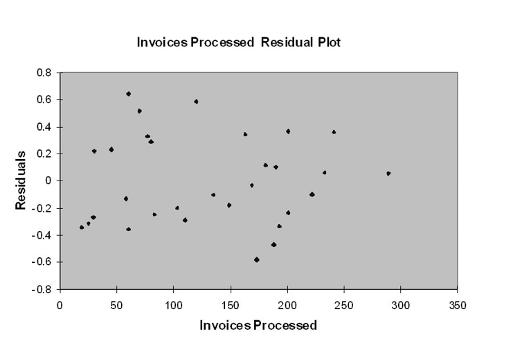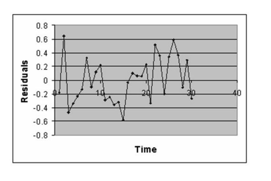TABLE 13- 11 Regression Statistics Multiple R 0.8531 RSquare 0.7278 Adjusted R Square 0.7180 Standard Error 47.8668 Observations 30 ANOVA d f SS MS F Significance F Regression 1 171499.78 171499.78 74.8505 2.1259E-09 Residual 28 64154.42 2291.23 Total 29 235654.20 Coefficients Standard Error t Stat p -value Lower 95\% Upper 95\% Intercept 76.5351 11.8318 6.4686 5.24-07 52.2987 100.7716 Gross 4.3331 0.5008 8.6516 2.13-09 3.3072 5.3590 -Referring to Table 13-12, what percentage of the variation in the amount of time needed can be explained by the variation in the number of invoices processed?

TABLE 13-2 A candy bar manufacturer is interested in trying to estimate how sales are influenced by the price of their product. To do this, the company randomly chooses 6 small cities and offers the candy bar at different prices. Using candy bar sales as the dependent variable, the company will conduct a simple linear regression on the data below: City Price (\ ) Sales River Falls 1.30 100 Hudson 1.60 90 Ellsworth 1.80 90 Prescott 2.00 40 Rock Elm 2.40 38 Stillwater 2.90 32 -Referring to Table 13-2, to test whether a change in price will have any impact on average sales, what would be the critical values? Use ? = 0.05.

TABLE 13-9 It is believed that, the average numbers of hours spent studying per day (HOURS) during undergraduate education should have a positive linear relationship with the starting salary (SALARY, measured in thousands of dollars per month) after graduation. Given below is the Excel output from regressing starting salary on number of hours spent studying per day for a sample of 51 students. NOTE: Some of the numbers in the output are purposely erased. Regression Statistics Multiple R 0.8857 R Square 0.7845 Adjusted R Square 0.7801 Standard Error 1.3704 Observations 51 $\text { ANOVA }$ df SS MS F Significance F Regression 1 335.0472 335.0473 178.3859 Residual 1.8782 Total 50 427.0798 -Referring to Table 13-9, the value of the measured t-test statistic to test whether average SALARY depends linearly on HOURS is Coefficients Standaad Error t Stat p -value Lower 95\% Upper 95\% Intercept -1.8940 0.4018 -4.7134 2.051-05 -2.7015 -1.0865 Hours 0.9795 0.0733 13.3561 5.944-18 0.8321 1.1269

TABLE 13-2 A candy bar manufacturer is interested in trying to estimate how sales are influenced by the price of their product. To do this, the company randomly chooses 6 small cities and offers the candy bar at different prices. Using candy bar sales as the dependent variable, the company will conduct a simple linear regression on the data below: City Price (\ ) Sales River Falls 1.30 100 Hudson 1.60 90 Ellsworth 1.80 90 Prescott 2.00 40 Rock Elm 2.40 38 Stillwater 2.90 32 -The sample correlation coefficient between X and Y is 0.375. It has been found out that the p- value is 0.744 when testing H0 : ? = 0 against the one- sided alternative H0 : ? < 0. To test H0 : ? = 0 against the two- sided alternative H0 : ?? 0 at a significance level of 0.2, the p- value is

TABLE 13-4 The managers of a brokerage firm are interested in finding out if the number of new clients a broker brings intothe firm affects the sales generated by the broker. Theysample 12 brokersand determine the numberof new clients they have enrolled in the last year and their sales amountsin thousandsof dollars. These data are presented in the table that follows. Broker Clients Sales 1 27 52 2 11 37 3 42 64 4 33 55 5 15 29 6 15 34 7 25 58 8 36 59 9 28 44 10 30 48 11 17 31 12 22 38 -Referring to Table 13-10, what is the value of the standard error of the estimate?

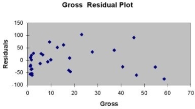
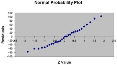
TABLE 13- 11 A company that has the distribution rights to home video sales of previously released movies would like to use the box office gross (in millions of dollars) to estimate the number of units (in thousands of units) that it can expect to sell. Following is the output from a simple linear regression along with the residual plot and normal probability plot obtained from a data set of 30 different movie titles: Regression Statistics Multiple R 0.8531 RSquare 0.7278 Adjusted R Square 0.7180 Standard Error 47.8668 Observations 30 ANOVA d f SS MS F Significance F Regression 1 171499.78 171499.78 74.8505 2.1259E-09 Residual 28 64154.42 2291.23 Total 29 235654.20 Coefficients Standard Error t Stat p -value Lower 95\% Upper 95\% Intercept 76.5351 11.8318 6.4686 5.24-07 52.2987 100.7716 Gross 4.3331 0.5008 8.6516 2.13-09 3.3072 5.3590 -Referring to Table 13-11, which of the following assumptions appears to have been violated?

TABLE 13-10 The management of a chain electronic store would like to develop a model for predicting the weekly sales (in thousand of dollars) for individual stores based on the number of customers who made purchases. A random sample of 12 stores yields the following results: Customers Sales (Thousands of Dollars) 907 11.20 926 11.05 713 8.21 741 9.21 780 9.42 898 10.08 510 6.73 529 7.02 460 6.12 872 9.52 650 7.53 603 7.25 -Referring to Table 13-10, what is the value of the coefficient of determination?

TABLE 13-12 The manager of the purchasing department of a large banking organization would like to develop a model to predict the amount of time (measured in hours) it takes to process invoices. Data are collected from a sample of 30 days, and the number of invoices processed and completion time in hours is recorded. Below is the regression output: Regression Statistics Multiple R 0.9947 R Square 0.8924 Adjusted R Square 0.8886 Standard Error 0.3342 ations 30 d f SS MS F Significance F Regression 1 25.9438 25.9438 232.2200 4.3946-15 Residual 28 3.1282 0.1117 Total 29 29.072 Coefficients Standard Error t Stat p -value Lower 95\% Upper 95\% Invoices 0.4024 0.1236 3.2559 0.0030 0.1492 0.6555 Processed 0.0126 0.0008 15.2388 4.3946-15 0.0109 0.0143 -Referring to Table 13-12, the model appears to be adequate based on the residual analyses.

If the correlation coefficient (r) = 1.00, then

TABLE 13-4 The managers of a brokerage firm are interested in finding out if the number of new clients a broker brings into the firm affects the sales generated by the broker. They sample 12 brokers and determine the number of new clients they have enrolled in the last year and their sales amounts in thousands of dollars. These data are presented in the table that follows. Broker Cliente Sales 1 27 52 2 11 37 3 42 64 4 33 55 5 15 29 6 15 34 7 25 58 8 36 59 9 28 44 10 30 48 11 17 31 12 22 38 -Referring to Table 13-4, suppose the managers of the brokerage firm want to obtain both a 99% confidence interval estimate and a 99% prediction interval for X = 24. The confidence interval estimate would be the_____ (wider or narrower) of the two intervals.

The standard error of the estimate is a measure of

TABLE 13-4 The managers of a brokerage firm are interested in finding out if the number of new clients a broker brings intothe firm affects the sales generated by the broker. Theysample 12 brokersand determine the numberof new clients they have enrolled in the last year and their sales amountsin thousandsof dollars. These data are presented in the table that follows. Broker Clients Sales 1 27 52 2 11 37 3 42 64 4 33 55 5 15 29 6 15 34 7 25 58 8 36 59 9 28 44 10 30 48 11 17 31 12 22 38 -Referring to Table 13-4, suppose the managers of the brokerage firm want to obtain a 99% prediction interval for the sales made by a broker who has brought into the firm 18 new clients. The prediction interval is from _____to _____.

$\text { TABLE 13-4 }$ The managers of a brokerage firm are interested in finding out if the number of new clients a broker brings into the firm affects the sales generated by the broker. They sample 12 brokers and determine the number of new clients they have enrolled in the last year and their sales amounts in thousands of dollars. These data are presented in the table that follows. Broker Clients Sales 1 27 52 2 11 37 3 42 64 4 33 55 5 15 29 6 15 34 7 25 58 8 36 59 9 28 44 10 30 48 11 17 31 12 22 38 -Referring to Table 13-4, the managers of the brokerage firm wanted to test the hypothesis that the number of new clients brought in did not affect the amount of sales generated. The value of the test statistic is _____ .

TABLE 13-2 A candy bar manufacturer is interested in trying to estimate how sales are influenced by the price of their product. To do this, the company randomly chooses 6 small cities and offers the candy bar at different prices. Using candy bar sales as the dependent variable, the company will conduct a simple linear regression on the data below: City Price (\ ) Sales River Falls 1.30 100 Hudson 1.60 90 Ellsworth 1.80 90 Prescott 2.00 40 Rock Elm 2.40 38 Stillwater 2.90 32 -Referring to Table 13-2, what is the estimated average change in the sales of the candy bar if price goes up by $1.00?

The Y-intercept (b₀) represents the

TABLE 13-9 It is believed that, the average numbers of hours spent studying per day (HOURS) during undergraduate education should have a positive linear relationship with the starting salary (SALARY, measured in thousands of dollars per month) after graduation. Given below is the Excel output from regressing starting salary on number of hours spent studying per day for a sample of 51 students. NOTE: Some of the numbers in the output are purposely erased. Regression Stedistics Multiple R 0.8857 RSquare 0.7845 Adjusted R Square 0.7801 Standard Error 1.3704 Observations 51 ANOVA df SS MS F Significance F Regression 1 335.0472 335.0473 178.3859 Residual 1.8782 Total 50 427.0798 Coeffcients Standard Error t Stat p- -value Lower 95\% Upper 95\% Intercept -1.8940 0.4018 -4.7134 2.051-05 -2.7015 -1.0865 Hours 0.9795 0.0733 13.3561 5.944-18 0.8321 1.1269 -Referring to Table 13-9, the p-value of the measured F-test statistic to test whether HOURS affects SALARY is

TABLE 13-4 The managers of a brokerage firm are interested in finding out if the number of new clients a broker brings intothe firm affects the sales generated by the broker. Theysample 12 brokersand determine the numberof new clients they have enrolled in the last year and their sales amountsin thousandsof dollars. These data are presented in the table that follows. Broker Clients Sales 1 27 52 2 11 37 3 42 64 4 33 55 5 15 29 6 15 34 7 25 58 8 36 59 9 28 44 10 30 48 11 17 31 12 22 38 -Referring to Table 13-4, the coefficient of correlation is_______ .

The sample correlation coefficient between X and Y is 0.375. It has been found out that the p-value is 0.256 when testing H₀ : ? = 0 against the two-sided alternative H₀ :? ? 0. To test H₀ : ? = 0 against the one-sided alternative H₀ : ? < 0 at a significance level of 0.2, the p-value is

TABLE 13-2 A candy bar manufacturer is interested in trying to estimate how sales are influenced by the price of their product. To do this, the company randomly chooses 6 small cities and offers the candy bar at different prices. Using candy bar sales as the dependent variable, the company will conduct a simple linear regression on the data below: City Price (\ ) Sales River Falls 1.30 100 Hudson 1.60 90 Ellsworth 1.80 90 Prescott 2.00 40 Rock Elm 2.40 38 Stillwater 2.90 32 -Referring to Table 13-2, if the price of the candy bar is set at $2, the predicted sales will be

The coefficient of determination (r²) tells us