Deck 11: Analysis of Variance
Full screen (f)
Question
Question
Question
Question
Question
Question
Question
Question
Question
Question
Question
TABLE 11-4
A campus researcher wanted to investigate the factors that affect visitor travel time in a complex, multilevel building on campus. Specifically, he wanted to determine whether different building signs (building maps versus wall signage) affect the total amount of time visitors require to reach their destination and whether that time depends on whether the starting location is inside or outside the building. Three subjects were assigned to each of the combinations of signs and starting locations, and travel time in seconds from beginning to destination was recorded. An Excel output of the appropriate analysis is given below:
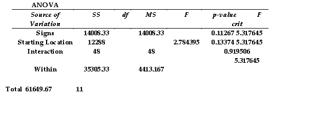
-Referring to Table 11-4, the degrees of freedom for the different building signs (factor A) is
A) 8.
B) 2.
C) 1.
D) 3.
A campus researcher wanted to investigate the factors that affect visitor travel time in a complex, multilevel building on campus. Specifically, he wanted to determine whether different building signs (building maps versus wall signage) affect the total amount of time visitors require to reach their destination and whether that time depends on whether the starting location is inside or outside the building. Three subjects were assigned to each of the combinations of signs and starting locations, and travel time in seconds from beginning to destination was recorded. An Excel output of the appropriate analysis is given below:
-Referring to Table 11-4, the degrees of freedom for the different building signs (factor A) is
A) 8.
B) 2.
C) 1.
D) 3.
Question
Question
Question
Question
Question
Question
Question
Question
Question
Question
Question
Question
Question
Question
Question
Question
Question
Question
TABLE 11-4
A campus researcher wanted to investigate the factors that affect visitor travel time in a complex, multilevel building on campus. Specifically, he wanted to determine whether different building signs (building maps versus wall signage) affect the total amount of time visitors require to reach their destination and whether that time depends on whether the starting location is inside or outside the building. Three subjects were assigned to each of the combinations of signs and starting locations, and travel time in seconds from beginning to destination was recorded. An Excel output of the appropriate analysis is given below:

-Referring to Table 11-4, the F test statistic for testing the interaction effect between the types of signs and the starting location is
A) 3.1742.
B) 5.3176.
C) 0.0109.
D) 2.7844.
A campus researcher wanted to investigate the factors that affect visitor travel time in a complex, multilevel building on campus. Specifically, he wanted to determine whether different building signs (building maps versus wall signage) affect the total amount of time visitors require to reach their destination and whether that time depends on whether the starting location is inside or outside the building. Three subjects were assigned to each of the combinations of signs and starting locations, and travel time in seconds from beginning to destination was recorded. An Excel output of the appropriate analysis is given below:
-Referring to Table 11-4, the F test statistic for testing the interaction effect between the types of signs and the starting location is
A) 3.1742.
B) 5.3176.
C) 0.0109.
D) 2.7844.
Question
TABLE 11-4
A campus researcher wanted to investigate the factors that affect visitor travel time in a complex, multilevel building on campus. Specifically, he wanted to determine whether different building signs (building maps versus wall signage) affect the total amount of time visitors require to reach their destination and whether that time depends on whether the starting location is inside or outside the building. Three subjects were assigned to each of the combinations of signs and starting locations, and travel time in seconds from beginning to destination was recorded. An Excel output of the appropriate analysis is given below:
-Referring to Table 11-4, the F test statistic for testing the main effect of types of signs is
A) 2.7844.
B) 0.0109.
C) 5.3176.
D) 3.1742.
Question
Question
TABLE 11-4
A campus researcher wanted to investigate the factors that affect visitor travel time in a complex, multilevel building on campus. Specifically, he wanted to determine whether different building signs (building maps versus wall signage) affect the total amount of time visitors require to reach their destination and whether that time depends on whether the starting location is inside or outside the building. Three subjects were assigned to each of the combinations of signs and starting locations, and travel time in seconds from beginning to destination was recorded. An Excel output of the appropriate analysis is given below:
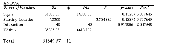
-Referring to Table 11-4, the mean squares for starting location (factor B) is
A) 14,008.3.
B) 4,413.17.
C) 12,288.
D) 48.
A campus researcher wanted to investigate the factors that affect visitor travel time in a complex, multilevel building on campus. Specifically, he wanted to determine whether different building signs (building maps versus wall signage) affect the total amount of time visitors require to reach their destination and whether that time depends on whether the starting location is inside or outside the building. Three subjects were assigned to each of the combinations of signs and starting locations, and travel time in seconds from beginning to destination was recorded. An Excel output of the appropriate analysis is given below:
-Referring to Table 11-4, the mean squares for starting location (factor B) is
A) 14,008.3.
B) 4,413.17.
C) 12,288.
D) 48.
Question
TABLE 11-4
A campus researcher wanted to investigate the factors that affect visitor travel time in a complex, multilevel building on campus. Specifically, he wanted to determine whether different building signs (building maps versus wall signage) affect the total amount of time visitors require to reach their destination and whether that time depends on whether the starting location is inside or outside the building. Three subjects were assigned to each of the combinations of signs and starting locations, and travel time in seconds from beginning to destination was recorded. An Excel output of the appropriate analysis is given below:

-Referring to Table 11-4, at 10% level of significance
A) there is sufficient evidence to conclude that the difference between the average traveling time for the different starting locations does not depend on the types of signs.
B) there is insufficient evidence to conclude that the difference between the average traveling time for the different types of signs depends on the starting locations.
C) there is sufficient evidence to conclude that the difference between the average traveling time for the different starting locations depends on the types of signs.
D) none of the above
A campus researcher wanted to investigate the factors that affect visitor travel time in a complex, multilevel building on campus. Specifically, he wanted to determine whether different building signs (building maps versus wall signage) affect the total amount of time visitors require to reach their destination and whether that time depends on whether the starting location is inside or outside the building. Three subjects were assigned to each of the combinations of signs and starting locations, and travel time in seconds from beginning to destination was recorded. An Excel output of the appropriate analysis is given below:
-Referring to Table 11-4, at 10% level of significance
A) there is sufficient evidence to conclude that the difference between the average traveling time for the different starting locations does not depend on the types of signs.
B) there is insufficient evidence to conclude that the difference between the average traveling time for the different types of signs depends on the starting locations.
C) there is sufficient evidence to conclude that the difference between the average traveling time for the different starting locations depends on the types of signs.
D) none of the above
Question
Question
Question
Question
TABLE 11-4
A campus researcher wanted to investigate the factors that affect visitor travel time in a complex, multilevel building on campus. Specifically, he wanted to determine whether different building signs (building maps versus wall signage) affect the total amount of time visitors require to reach their destination and whether that time depends on whether the starting location is inside or outside the building. Three subjects were assigned to each of the combinations of signs and starting locations, and travel time in seconds from beginning to destination was recorded. An Excel output of the appropriate analysis is given below:
-Referring to Table 11-4, the within (error) degrees of freedom is
A) 1.
B) 11.
C) 8.
D) 4.
Question
Question
Question
Question
TABLE 11-6
As part of an evaluation program, a sporting goods retailer wanted to compare the downhill coasting speeds of 4 brands of bicycles. She took 3 of each brand and determined their maximum downhill speeds. The results are presented in miles per hour in the table below.

Referring to Table 11-6, what is the p-value of the test statistic for Levene's test for homogeneity of variances?
As part of an evaluation program, a sporting goods retailer wanted to compare the downhill coasting speeds of 4 brands of bicycles. She took 3 of each brand and determined their maximum downhill speeds. The results are presented in miles per hour in the table below.
Referring to Table 11-6, what is the p-value of the test statistic for Levene's test for homogeneity of variances?
Question
Question
Question
Question
Question
Question
Question
Question
Question
Question
Question
Question
Question
Question
Question
Question
Question
Question
Question
Question
Question
Question
Question
Question
Question
Question
Question
Question
TABLE 11-11
A student team in a business statistics course designed an experiment to investigate whether the brand of bubblegum used affected the size of bubbles they could blow. To reduce the person-to-person variability, the students decided to use a randomized block design using themselves as blocks. Four brands of bubblegum were tested. A student chewed two pieces of a brand of gum and then blew a bubble, attempting to make it as big as possible. Another student measured the diameter of the bubble at its biggest point. The following table gives the diameters of the bubbles (in inches) for the 16 observations.

Referring to Table 11-11, what are the degrees of freedom of the F test statistic for testing the block effects?
A student team in a business statistics course designed an experiment to investigate whether the brand of bubblegum used affected the size of bubbles they could blow. To reduce the person-to-person variability, the students decided to use a randomized block design using themselves as blocks. Four brands of bubblegum were tested. A student chewed two pieces of a brand of gum and then blew a bubble, attempting to make it as big as possible. Another student measured the diameter of the bubble at its biggest point. The following table gives the diameters of the bubbles (in inches) for the 16 observations.
Referring to Table 11-11, what are the degrees of freedom of the F test statistic for testing the block effects?
Question
Question
Question
Question
Question
Question
Question
Question
TABLE 11-8
A hotel chain has identically sized resorts in 5 locations. The data that follow resulted from analyzing the hotel occupancies on randomly selected days in the 5 locations.

Referring to Table 11-8, what are the numerator and denominator degrees of freedom for Levene's test for homogeneity of variances respectively?
A hotel chain has identically sized resorts in 5 locations. The data that follow resulted from analyzing the hotel occupancies on randomly selected days in the 5 locations.
Referring to Table 11-8, what are the numerator and denominator degrees of freedom for Levene's test for homogeneity of variances respectively?
Question
Question
Question

Unlock Deck
Sign up to unlock the cards in this deck!
Unlock Deck
Unlock Deck
1/179
Play
Full screen (f)
Deck 11: Analysis of Variance
1
TABLE 11-2
An airline wants to select a computer software package for its reservation system. Four software packages (1, 2, 3, and 4) are commercially available. The airline will choose the package that bumps as few passengers, on the average, as possible during a month. An experiment is set up in which each package is used to make reservations for 5 randomly selected weeks. (A total of 20 weeks was included in the experiment.) The number of passengers bumped each week is obtained, which gives rise to the following Excel output:
-Referring to Table 11-2, the within group degrees of freedom is
A) 4.
B) 3.
C) 19.
D) 16.
16.
2
TABLE 11-5
A physician and president of a Tampa Health Maintenance Organization (HMO) are attempting to show the benefits of managed health care to an insurance company. The physician believes that certain types of doctors are more cost-effective than others. One theory is that Primary Specialty is an important factor in measuring the cost-effectiveness of physicians. To investigate this, the president obtained independent random samples of 20 HMO physicians from each of 4 primary specialties - General Practice (GP), Internal Medicine (IM), Pediatrics (PED), and Family Physicians (FP) - and recorded the total charges per member per month for each. A second factor which the president believes influences total charges per member per month is whether the doctor is a foreign or USA medical school graduate. The president theorizes that foreign graduates will have higher mean charges than USA graduates. To investigate this, the president also collected data on 20 foreign medical school graduates in each of the 4 primary specialty types described above. So information on charges for 40 doctors (20 foreign and 20 USA medical school graduates) was obtained for each of the 4 specialties. The results for the ANOVA are summarized in the following table.
-Referring to Table 11-5, what degrees of freedom should be used to determine the critical value of the F ratio against which to test for differences between the mean charges of foreign and USA medical school graduates?
A) numerator df = 1, denominator df = 152
B) numerator df = 3, denominator df = 159
C) numerator df = 3, denominator df = 152
D) numerator df = 1, denominator df = 159
numerator df = 1, denominator df = 152
3
An airline wants to select a computer software package for its reservation system. Four software packages (1, 2, 3, and 4) are commercially available. The airline will choose the package that bumps as few passengers, on the average, as possible during a month. An experiment is set up in which each package is used to make reservations for 5 randomly selected weeks. (A total of 20 weeks was included in the experiment.) The number of passengers bumped each week is obtained, which gives rise to the following Excel output:
-Referring to Table 11-2, the total degrees of freedom is
A) 3.
B) 16.
C) 4.
D) 19.
-Referring to Table 11-2, the total degrees of freedom is
A) 3.
B) 16.
C) 4.
D) 19.
19.
4
TABLE 11-3
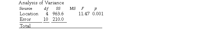
A realtor wants to compare the average sales-to-appraisal ratios of residential properties sold in four neighborhoods (A, B, C, and D). Four properties are randomly selected from each neighborhood and the ratios recorded for each, as shown below.
A: C:
B: D:
Interpret the results of the analysis summarized in the following table:
-Referring to Table 11-3,
A) at the 0.05 level of significance, the mean ratios for the 4 neighborhoods are not all the same.
B) at the 0.10 level of significance, the mean ratios for the 4 neighborhoods are not significantly different.
C) at the 0.01 level of significance, the mean ratios for the 4 neighborhoods are all the same.
D) at the 0.05 level of significance, the mean ratios for the 4 neighborhoods are not significantly different from 0.
Unlock Deck
Unlock for access to all 179 flashcards in this deck.
Unlock Deck
k this deck
5
TABLE 11-6
As part of an evaluation program, a sporting goods retailer wanted to compare the downhill coasting speeds of 4 brands of bicycles. She took 3 of each brand and determined their maximum downhill speeds. The results are presented in miles per hour in the table below.
-Referring to Table 11-6, what should be the conclusion for the Levene's test for homogeneity of variances at a 5% level of significance?
A) There is not sufficient evidence that the variances are not all the same.
B) There is sufficient evidence that the variances are not all the same.
C) There is not sufficient evidence that the variances are all the same.
D) There is sufficient evidence that the variances are all the same.
Unlock Deck
Unlock for access to all 179 flashcards in this deck.
Unlock Deck
k this deck
6
TABLE 11-5
A physician and president of a Tampa Health Maintenance Organization (HMO) are attempting to show the benefits of managed health care to an insurance company. The physician believes that certain types of doctors are more cost-effective than others. One theory is that Primary Specialty is an important factor in measuring the cost-effectiveness of physicians. To investigate this, the president obtained independent random samples of 20 HMO physicians from each of 4 primary specialties - General Practice (GP), Internal Medicine (IM), Pediatrics (PED), and Family Physicians (FP) - and recorded the total charges per member per month for each. A second factor which the president believes influences total charges per member per month is whether the doctor is a foreign or USA medical school graduate. The president theorizes that foreign graduates will have higher mean charges than USA graduates. To investigate this, the president also collected data on 20 foreign medical school graduates in each of the 4 primary specialty types described above. So information on charges for 40 doctors (20 foreign and 20 USA medical school graduates) was obtained for each of the 4 specialties. The results for the ANOVA are summarized in the following table.
-Referring to Table 11-5, what was the total number of doctors included in the study?
A) 160
B) 159
C) 20
D) 40
Unlock Deck
Unlock for access to all 179 flashcards in this deck.
Unlock Deck
k this deck
7
TABLE 11-5
A physician and president of a Tampa Health Maintenance Organization (HMO) are attempting to show the benefits of managed health care to an insurance company. The physician believes that certain types of doctors are more cost-effective than others. One theory is that Primary Specialty is an important factor in measuring the cost-effectiveness of physicians. To investigate this, the president obtained independent random samples of 20 HMO physicians from each of 4 primary specialties - General Practice (GP), Internal Medicine (IM), Pediatrics (PED), and Family Physicians (FP) - and recorded the total charges per member per month for each. A second factor which the president believes influences total charges per member per month is whether the doctor is a foreign or USA medical school graduate. The president theorizes that foreign graduates will have higher mean charges than USA graduates. To investigate this, the president also collected data on 20 foreign medical school graduates in each of the 4 primary specialty types described above. So information on charges for 40 doctors (20 foreign and 20 USA medical school graduates) was obtained for each of the 4 specialties. The results for the ANOVA are summarized in the following table.
-Referring to Table 11-5, is there evidence of a difference between the mean charges of foreign and USA medical school graduates?
A) No, the test for the main effect for medical school is not significant at ? = 0.10.
B) Maybe, but we need information on the þ-estimates to fully answer the question.
C) Yes, the test for the main effect for primary specialty is significant at ? = 0.10.
D) No, the test for the interaction is not significant at ? = 0.10.
Unlock Deck
Unlock for access to all 179 flashcards in this deck.
Unlock Deck
k this deck
8
Why would you use the Tukey-Kramer procedure?
A) to test for differences in pairwise means
B) to test independence of errors
C) to test for homogeneity of variance
D) to test for normality
A) to test for differences in pairwise means
B) to test independence of errors
C) to test for homogeneity of variance
D) to test for normality
Unlock Deck
Unlock for access to all 179 flashcards in this deck.
Unlock Deck
k this deck
9
TABLE 11-3
A realtor wants to compare the average sales-to-appraisal ratios of residential properties sold in four neighborhoods (A, B, C, and D). Four properties are randomly selected from each neighborhood and the ratios recorded for each, as shown below.
A: 1.2, 1.1, 0.9, 0.4 C: 1.0, 1.5, 1.1, 1.3
B: 2.5, 2.1, 1.9, 1.6 D: 0.8, 1.3, 1.1, 0.7
Interpret the results of the analysis summarized in the following table:
-Referring to Table 11-3, the among group degrees of freedom is
A) 12.
B) 16.
C) 4.
D) 3.
Unlock Deck
Unlock for access to all 179 flashcards in this deck.
Unlock Deck
k this deck
10
TABLE 11-6
As part of an evaluation program, a sporting goods retailer wanted to compare the downhill coasting speeds of 4 brands of bicycles. She took 3 of each brand and determined their maximum downhill speeds. The results are presented in miles per hour in the table below.
-Referring to Table 11-6, what should be the decision for the Levene's test for homogeneity of variances at a 5% level of significance?
A) Do not reject the null hypothesis because the p-value is larger than the level of significance.
B) Reject the null hypothesis because the p-value is larger than the level of significance.
C) Do not reject the null hypothesis because the p-value is smaller than the level of significance.
D) Reject the null hypothesis because the p-value is smaller than the level of significance.
Unlock Deck
Unlock for access to all 179 flashcards in this deck.
Unlock Deck
k this deck
11
TABLE 11-4
A campus researcher wanted to investigate the factors that affect visitor travel time in a complex, multilevel building on campus. Specifically, he wanted to determine whether different building signs (building maps versus wall signage) affect the total amount of time visitors require to reach their destination and whether that time depends on whether the starting location is inside or outside the building. Three subjects were assigned to each of the combinations of signs and starting locations, and travel time in seconds from beginning to destination was recorded. An Excel output of the appropriate analysis is given below:
-Referring to Table 11-4, the degrees of freedom for the different building signs (factor A) is
A) 8.
B) 2.
C) 1.
D) 3.
Unlock Deck
Unlock for access to all 179 flashcards in this deck.
Unlock Deck
k this deck
12
Which of the following components in an ANOVA table are not additive?
A) sum of squares
B) mean squares
C) degrees of freedom
D) It is not possible to tell.
A) sum of squares
B) mean squares
C) degrees of freedom
D) It is not possible to tell.
Unlock Deck
Unlock for access to all 179 flashcards in this deck.
Unlock Deck
k this deck
13
An airline wants to select a computer software package for its reservation system. Four software packages (1, 2, 3, and 4) are commercially available. The airline will choose the package that bumps as few passengers, on the average, as possible during a month. An experiment is set up in which each package is used to make reservations for 5 randomly selected weeks. (A total of 20 weeks was included in the experiment.) The number of passengers bumped each week is given below. How should the data be analyzed?
Package 1: 12, 14, 9, 11, 16
Package 2: 2, 4, 7, 3, 1
Package 3: 10, 9, 6, 10, 12
Package 4: 7, 6, 6, 15, 12
A) t test for the mean difference
B) t test for the differences in means
C) one-way ANOVA F test
D) F test for differences in variances
Package 1: 12, 14, 9, 11, 16
Package 2: 2, 4, 7, 3, 1
Package 3: 10, 9, 6, 10, 12
Package 4: 7, 6, 6, 15, 12
A) t test for the mean difference
B) t test for the differences in means
C) one-way ANOVA F test
D) F test for differences in variances
Unlock Deck
Unlock for access to all 179 flashcards in this deck.
Unlock Deck
k this deck
14
TABLE 11-11
A student team in a business statistics course designed an experiment to investigate whether the brand of bubblegum used affected the size of bubbles they could blow. To reduce the person-to-person variability, the students decided to use a randomized block design using themselves as blocks. Four brands of bubblegum were tested. A student chewed two pieces of a brand of gum and then blew a bubble, attempting to make it as big as possible. Another student measured the diameter of the bubble at its biggest point. The following table gives the diameters of the bubbles (in inches) for the 16 observations.
-Referring to Table 11-11, what is the null hypothesis for the randomized block F test for the difference in the means?
A) H0 : µKyle = µSarah = µLeigh = µIsaac
B) H0 : MA = MB = MC = MD
C) H0 : µA = µB = µC = µD
D) H0 : MKyle = MSarah = MLeigh = MIsaac
Unlock Deck
Unlock for access to all 179 flashcards in this deck.
Unlock Deck
k this deck
15
In a one-way ANOVA, if the computed F statistic exceeds the critical F value we may
A) not reject H0 because a mistake has been made.
B) reject H0 since there is evidence of a treatment effect.
C) not reject H0 since there is no evidence of a difference.
D) reject H0 since there is evidence all the means differ.
A) not reject H0 because a mistake has been made.
B) reject H0 since there is evidence of a treatment effect.
C) not reject H0 since there is no evidence of a difference.
D) reject H0 since there is evidence all the means differ.
Unlock Deck
Unlock for access to all 179 flashcards in this deck.
Unlock Deck
k this deck
16
In a one-way ANOVA, the null hypothesis is always
A) all the population means are different.
B) there is no treatment effect.
C) there is some treatment effect.
D) some of the population means are different.
A) all the population means are different.
B) there is no treatment effect.
C) there is some treatment effect.
D) some of the population means are different.
Unlock Deck
Unlock for access to all 179 flashcards in this deck.
Unlock Deck
k this deck
17
Interaction in an experimental design can be tested in
A) a two-factor model.
B) a randomized block model.
C) all ANOVA models.
D) a completely randomized model.
A) a two-factor model.
B) a randomized block model.
C) all ANOVA models.
D) a completely randomized model.
Unlock Deck
Unlock for access to all 179 flashcards in this deck.
Unlock Deck
k this deck
18
A campus researcher wanted to investigate the factors that affect visitor travel time in a complex, multilevel building on campus. Specifically, he wanted to determine whether different building signs (building maps versus wall signage) affect the total amount of time visitors require to reach their destination and whether that time depends on whether the starting location is inside or outside the building. Three subjects were assigned to each of the combinations of signs and starting locations, and travel time in seconds from beginning to destination was recorded. How should the data be analyzed?
A) 2 × 2 factorial design
B) completely randomized design
C) randomized block design
D) levene's test
A) 2 × 2 factorial design
B) completely randomized design
C) randomized block design
D) levene's test
Unlock Deck
Unlock for access to all 179 flashcards in this deck.
Unlock Deck
k this deck
19
TABLE 11-5
A physician and president of a Tampa Health Maintenance Organization (HMO) are attempting to show the benefits of managed health care to an insurance company. The physician believes that certain types of doctors are more cost-effective than others. One theory is that Primary Specialty is an important factor in measuring the cost-effectiveness of physicians. To investigate this, the president obtained independent random samples of 20 HMO physicians from each of 4 primary specialties - General Practice (GP), Internal Medicine (IM), Pediatrics (PED), and Family Physicians (FP) - and recorded the total charges per member per month for each. A second factor which the president believes influences total charges per member per month is whether the doctor is a foreign or USA medical school graduate. The president theorizes that foreign graduates will have higher mean charges than USA graduates. To investigate this, the president also collected data on 20 foreign medical school graduates in each of the 4 primary specialty types described above. So information on charges for 40 doctors (20 foreign and 20 USA medical school graduates) was obtained for each of the 4 specialties. The results for the ANOVA are summarized in the following table.
-Referring to Table 11-5, what degrees of freedom should be used to determine the critical value of the F ratio against which to test for interaction between the two factors?
A) numerator df = 3, denominator df = 152
B) numerator df = 3, denominator df = 159
C) numerator df = 1, denominator df = 152
D) numerator df = 1, denominator df = 159
Unlock Deck
Unlock for access to all 179 flashcards in this deck.
Unlock Deck
k this deck
20
TABLE 11-5
A physician and president of a Tampa Health Maintenance Organization (HMO) are attempting to show the benefits of managed health care to an insurance company. The physician believes that certain types of doctors are more cost-effective than others. One theory is that Primary Specialty is an important factor in measuring the cost-effectiveness of physicians. To investigate this, the president obtained independent random samples of 20 HMO physicians from each of 4 primary specialties - General Practice (GP), Internal Medicine (IM), Pediatrics (PED), and Family Physicians (FP) - and recorded the total charges per member per month for each. A second factor which the president believes influences total charges per member per month is whether the doctor is a foreign or USA medical school graduate. The president theorizes that foreign graduates will have higher mean charges than USA graduates. To investigate this, the president also collected data on 20 foreign medical school graduates in each of the 4 primary specialty types described above. So information on charges for 40 doctors (20 foreign and 20 USA medical school graduates) was obtained for each of the 4 specialties. The results for the ANOVA are summarized in the following table.
-Referring to Table 11-5, interpret the test for interaction.
A) There is sufficient evidence to say at the 0.10 level of significance that mean charges depend on both primary specialty and medical school.
B) There is insufficient evidence to say at the 0.10 level of significance that the difference between the mean charges for foreign and USA graduates depends on primary specialty.
C) There is sufficient evidence to say at the 0.10 level of significance that the difference between the mean charges for foreign and USA graduates depends on primary specialty.
D) There is sufficient evidence at the 0.10 level of significance of a difference between the mean charges for foreign and USA medical graduates.
Unlock Deck
Unlock for access to all 179 flashcards in this deck.
Unlock Deck
k this deck
21
TABLE 11-3
A realtor wants to compare the average sales-to-appraisal ratios of residential properties sold in four neighborhoods (A, B, C, and D). Four properties are randomly selected from each neighborhood and the ratios recorded for each, as shown below.
A: C:
B: D:
Interpret the results of the analysis summarized in the following table:
-Referring to Table 11-3, the within group sum of squares is
A) 3.1819.
B) 1.0606.
C) 1.1825.
D) 4.3644.
Unlock Deck
Unlock for access to all 179 flashcards in this deck.
Unlock Deck
k this deck
22
TABLE 11-8
A hotel chain has identically sized resorts in 5 locations. The data that follow resulted from analyzing the hotel occupancies on randomly selected days in the 5 locations.
-Referring to Table 11-8, what is the null hypothesis for Levene's test for homogeneity of variances?
A)
B)
C) H0 : MA = MB = MC = MD
D)
Unlock Deck
Unlock for access to all 179 flashcards in this deck.
Unlock Deck
k this deck
23
TABLE 11-4
A campus researcher wanted to investigate the factors that affect visitor travel time in a complex, multilevel building on campus. Specifically, he wanted to determine whether different building signs (building maps versus wall signage) affect the total amount of time visitors require to reach their destination and whether that time depends on whether the starting location is inside or outside the building. Three subjects were assigned to each of the combinations of signs and starting locations, and travel time in seconds from beginning to destination was recorded. An Excel output of the appropriate analysis is given below:
-Referring to Table 11-4, at 1% level of significance
A) there is insufficient evidence to conclude that the relationship between traveling time and the types of signs depends on the starting locations.
B) there is insufficient evidence to conclude that the difference between the average traveling time for the different starting locations depends on the types of signs.
C) there is insufficient evidence to conclude that the difference between the average traveling time for the different types of signs depends on the starting locations.
D) all of the above
Unlock Deck
Unlock for access to all 179 flashcards in this deck.
Unlock Deck
k this deck
24
TABLE 11-8
A hotel chain has identically sized resorts in 5 locations. The data that follow resulted from analyzing the hotel occupancies on randomly selected days in the 5 locations.
-Referring to Table 11-8, what should be the decision for the Levene's test for homogeneity of variances at a 5% level of significance?
A) Do not reject the null hypothesis because the p-value is larger than the level of significance.
B) Reject the null hypothesis because the p-value is larger than the level of significance.
C) Reject the null hypothesis because the p-value is smaller than the level of significance.
D) Do not reject the null hypothesis because the p-value is smaller than the level of significance.
Unlock Deck
Unlock for access to all 179 flashcards in this deck.
Unlock Deck
k this deck
25
An airline wants to select a computer software package for its reservation system. Four software packages (1, 2, 3, and 4) are commercially available. The airline will choose the package that bumps as few passengers, on the average, as possible during a month. An experiment is set up in which each package is used to make reservations for 5 randomly selected weeks. (A total of 20 weeks was included in the experiment.) The number of passengers bumped each week is obtained, which gives rise to the following Excel output:
-Referring to Table 11-2, at a significance level of 1%
A) there is sufficient evidence to conclude that the average numbers of customers bumped by the 4 packages are not all the same.
B) there is insufficient evidence to conclude that the average numbers of customers bumped by the 4 packages are not all the same.
C) there is sufficient evidence to conclude that the average numbers of customers bumped by the 4 packages are all the same.
D) there is insufficient evidence to conclude that the average numbers of customers bumped by the 4 packages are all the same.
Unlock Deck
Unlock for access to all 179 flashcards in this deck.
Unlock Deck
k this deck
26
TABLE 11-3
A realtor wants to compare the average sales-to-appraisal ratios of residential properties sold in four neighborhoods (A, B, C, and D). Four properties are randomly selected from each neighborhood and the ratios recorded for each, as shown below.
A: C:
B: D:
Interpret the results of the analysis summarized in the following table:
-Referring to Table 11-3, what is the null hypothesis for Levene's test for homogeneity of variances?
A)
B) H0 : MA = MB = MC = MD
C)
D) H0 : µA = µB = µC = µD
Unlock Deck
Unlock for access to all 179 flashcards in this deck.
Unlock Deck
k this deck
27
TABLE 11-2
An airline wants to select a computer software package for its reservation system. Four software packages (1, 2, 3, and 4) are commercially available. The airline will choose the package that bumps as few passengers, on the average, as possible during a month. An experiment is set up in which each package is used to make reservations for 5 randomly selected weeks. (A total of 20 weeks was included in the experiment.) The number of passengers bumped each week is obtained, which gives rise to the following Excel output:
-Referring to Table 11-2, the among-group (between-group) mean squares is
A) 70.8.
B) 212.4.
C) 8.525.
D) 637.2.
Unlock Deck
Unlock for access to all 179 flashcards in this deck.
Unlock Deck
k this deck
28
TABLE 11-5
A physician and president of a Tampa Health Maintenance Organization (HMO) are attempting to show the benefits of managed health care to an insurance company. The physician believes that certain types of doctors are more cost-effective than others. One theory is that Primary Specialty is an important factor in measuring the cost-effectiveness of physicians. To investigate this, the president obtained independent random samples of 20 HMO physicians from each of 4 primary specialties - General Practice (GP), Internal Medicine (IM), Pediatrics (PED), and Family Physicians (FP) - and recorded the total charges per member per month for each. A second factor which the president believes influences total charges per member per month is whether the doctor is a foreign or USA medical school graduate. The president theorizes that foreign graduates will have higher mean charges than USA graduates. To investigate this, the president also collected data on 20 foreign medical school graduates in each of the 4 primary specialty types described above. So information on charges for 40 doctors (20 foreign and 20 USA medical school graduates) was obtained for each of the 4 specialties. The results for the ANOVA are summarized in the following table.
-Referring to Table 11-5, what degrees of freedom should be used to determine the critical value of the F ratio against which to test for differences in the mean charges for doctors among the four primary specialty areas?
A) numerator df = 3, denominator df = 159
B) numerator df = 3, denominator df = 152
C) numerator df = 1, denominator df = 159
D) numerator df = 1, denominator df = 152
Unlock Deck
Unlock for access to all 179 flashcards in this deck.
Unlock Deck
k this deck
29
TABLE 11-4
A campus researcher wanted to investigate the factors that affect visitor travel time in a complex, multilevel building on campus. Specifically, he wanted to determine whether different building signs (building maps versus wall signage) affect the total amount of time visitors require to reach their destination and whether that time depends on whether the starting location is inside or outside the building. Three subjects were assigned to each of the combinations of signs and starting locations, and travel time in seconds from beginning to destination was recorded. An Excel output of the appropriate analysis is given below:
-Referring to Table 11-4, the F test statistic for testing the interaction effect between the types of signs and the starting location is
A) 3.1742.
B) 5.3176.
C) 0.0109.
D) 2.7844.
Unlock Deck
Unlock for access to all 179 flashcards in this deck.
Unlock Deck
k this deck
30
TABLE 11-4
A campus researcher wanted to investigate the factors that affect visitor travel time in a complex, multilevel building on campus. Specifically, he wanted to determine whether different building signs (building maps versus wall signage) affect the total amount of time visitors require to reach their destination and whether that time depends on whether the starting location is inside or outside the building. Three subjects were assigned to each of the combinations of signs and starting locations, and travel time in seconds from beginning to destination was recorded. An Excel output of the appropriate analysis is given below:
-Referring to Table 11-4, the F test statistic for testing the main effect of types of signs is
A) 2.7844.
B) 0.0109.
C) 5.3176.
D) 3.1742.
Unlock Deck
Unlock for access to all 179 flashcards in this deck.
Unlock Deck
k this deck
31
TABLE 11-6
As part of an evaluation program, a sporting goods retailer wanted to compare the downhill coasting speeds of 4 brands of bicycles. She took 3 of each brand and determined their maximum downhill speeds. The results are presented in miles per hour in the table below.
-Referring to Table 11-6, what is the null hypothesis for Levene's test for homogeneity of variances?
A) H0 : MA = MB = MC = MD
B)
C)
D)
Unlock Deck
Unlock for access to all 179 flashcards in this deck.
Unlock Deck
k this deck
32
TABLE 11-4
A campus researcher wanted to investigate the factors that affect visitor travel time in a complex, multilevel building on campus. Specifically, he wanted to determine whether different building signs (building maps versus wall signage) affect the total amount of time visitors require to reach their destination and whether that time depends on whether the starting location is inside or outside the building. Three subjects were assigned to each of the combinations of signs and starting locations, and travel time in seconds from beginning to destination was recorded. An Excel output of the appropriate analysis is given below:
-Referring to Table 11-4, the mean squares for starting location (factor B) is
A) 14,008.3.
B) 4,413.17.
C) 12,288.
D) 48.
Unlock Deck
Unlock for access to all 179 flashcards in this deck.
Unlock Deck
k this deck
33
TABLE 11-4
A campus researcher wanted to investigate the factors that affect visitor travel time in a complex, multilevel building on campus. Specifically, he wanted to determine whether different building signs (building maps versus wall signage) affect the total amount of time visitors require to reach their destination and whether that time depends on whether the starting location is inside or outside the building. Three subjects were assigned to each of the combinations of signs and starting locations, and travel time in seconds from beginning to destination was recorded. An Excel output of the appropriate analysis is given below:
-Referring to Table 11-4, at 10% level of significance
A) there is sufficient evidence to conclude that the difference between the average traveling time for the different starting locations does not depend on the types of signs.
B) there is insufficient evidence to conclude that the difference between the average traveling time for the different types of signs depends on the starting locations.
C) there is sufficient evidence to conclude that the difference between the average traveling time for the different starting locations depends on the types of signs.
D) none of the above
Unlock Deck
Unlock for access to all 179 flashcards in this deck.
Unlock Deck
k this deck
34
Psychologists have found that people are generally reluctant to transmit bad news to their peers. This phenomenon has been termed the "MUM effect." To investigate the cause of the MUM effect, 40 undergraduates at Duke University participated in an experiment. Each subject was asked to administer an IQ test to another student and then provide the test taker with his or her percentile score. Unknown to the subject, the test taker was a bogus student who was working with the researchers. The experimenters manipulated two factors: subject visibility and success of test taker, each at two levels. Subject visibility was either visible or not visible to the test taker. Success of the test taker was either top 20% or bottom 20%. Ten subjects were randomly assigned to each of the 2 x 2 = 4 experimental conditions, then the time (in seconds) between the end of the test and the delivery of the percentile score from the subject to the test taker was measured. (This variable is called the latency to feedback.) The data were subjected to appropriate analyses with the following results.
-Referring to Table 11-1, at the 0.01 level, what conclusions can you draw from the analysis?
A) At the 0.01 level, there is evidence to indicate that subject visibility and test taker success interact.
B) At the 0.01 level, subject visibility and test taker success are significant predictors of latency feedback.
C) At the 0.01 level, the model is not useful for predicting latency to feedback.
D) At the 0.01 level, there is no evidence of interaction between subject visibility and test taker success.
Unlock Deck
Unlock for access to all 179 flashcards in this deck.
Unlock Deck
k this deck
35
The degrees of freedom for the F test in a one-way ANOVA are
A) (c - n) and (n - 1).
B) (n - c) and (c - 1).
C) (c - 1) and (n - c).
D) (n - 1) and (c - n).
A) (c - n) and (n - 1).
B) (n - c) and (c - 1).
C) (c - 1) and (n - c).
D) (n - 1) and (c - n).
Unlock Deck
Unlock for access to all 179 flashcards in this deck.
Unlock Deck
k this deck
36
A realtor wants to compare the average sales-to-appraisal ratios of residential properties sold in four neighborhoods (A, B, C, and D). Four properties are randomly selected from each neighborhood and the ratios recorded for each, as shown below.
A: C:
B: D:
Interpret the results of the analysis summarized in the following table:
-Referring to Table 11-3, what should be the decision for the Levene's test for homogeneity of variances at a 5% level of significance?
A) Reject the null hypothesis because the p-value is larger than the level of significance.
B) Do not eject the null hypothesis because the p-value is smaller than the level of significance.
C) Reject the null hypothesis because the p-value is smaller than the level of significance.
D) Do not reject the null hypothesis because the p-value is larger than the level of significance.
Unlock Deck
Unlock for access to all 179 flashcards in this deck.
Unlock Deck
k this deck
37
TABLE 11-4
A campus researcher wanted to investigate the factors that affect visitor travel time in a complex, multilevel building on campus. Specifically, he wanted to determine whether different building signs (building maps versus wall signage) affect the total amount of time visitors require to reach their destination and whether that time depends on whether the starting location is inside or outside the building. Three subjects were assigned to each of the combinations of signs and starting locations, and travel time in seconds from beginning to destination was recorded. An Excel output of the appropriate analysis is given below:
-Referring to Table 11-4, the within (error) degrees of freedom is
A) 1.
B) 11.
C) 8.
D) 4.
Unlock Deck
Unlock for access to all 179 flashcards in this deck.
Unlock Deck
k this deck
38
A student team in a business statistics course designed an experiment to investigate whether the brand of bubblegum used affected the size of bubbles they could blow. To reduce the person-to-person variability, the students decided to use a randomized block design using themselves as blocks. Four brands of bubblegum were tested. A student chewed two pieces of a brand of gum and then blew a bubble, attempting to make it as big as possible. Another student measured the diameter of the bubble at its biggest point. The following table gives the diameters of the bubbles (in inches) for the 16 observations.
-Referring to Table 11-11, what is the null hypothesis for testing the block effects?
A) H0 : MKyle = MSarah = MLeigh = MIsaac
B) H0 : µKyle = µSarah = µLeigh = µIsaac
C) H0 : µA = µB = µC = µD D) H0 : MA = MB = MC = MD
-Referring to Table 11-11, what is the null hypothesis for testing the block effects?
A) H0 : MKyle = MSarah = MLeigh = MIsaac
B) H0 : µKyle = µSarah = µLeigh = µIsaac
C) H0 : µA = µB = µC = µD D) H0 : MA = MB = MC = MD
Unlock Deck
Unlock for access to all 179 flashcards in this deck.
Unlock Deck
k this deck
39
TABLE 11-8
A hotel chain has identically sized resorts in 5 locations. The data that follow resulted from analyzing the hotel occupancies on randomly selected days in the 5 locations.
-Referring to Table 11-8, what should be the conclusion for the Levene's test for homogeneity of variances at a 5% level of significance?
A) There is not sufficient evidence that the variances are not all the same.
B) There is sufficient evidence that the variances are not all the same.
C) There is not sufficient evidence that the variances are all the same.
D) There is sufficient evidence that the variances are all the same.
Unlock Deck
Unlock for access to all 179 flashcards in this deck.
Unlock Deck
k this deck
40
The F test statistic in a one-way ANOVA is
A) SSW/SSA.
B) MSA/MSW.
C) SSA/SSW.
D) MSW/MSA.
A) SSW/SSA.
B) MSA/MSW.
C) SSA/SSW.
D) MSW/MSA.
Unlock Deck
Unlock for access to all 179 flashcards in this deck.
Unlock Deck
k this deck
41
TABLE 11-6
As part of an evaluation program, a sporting goods retailer wanted to compare the downhill coasting speeds of 4 brands of bicycles. She took 3 of each brand and determined their maximum downhill speeds. The results are presented in miles per hour in the table below.
Referring to Table 11-6, what is the p-value of the test statistic for Levene's test for homogeneity of variances?
Unlock Deck
Unlock for access to all 179 flashcards in this deck.
Unlock Deck
k this deck
42
A physician and president of a Tampa Health Maintenance Organization (HMO) are attempting to show the benefits of managed health care to an insurance company. The physician believes that certain types of doctors are more cost-effective than others. One theory is that Primary Specialty is an important factor in measuring the cost-effectiveness of physicians. To investigate this, the president obtained independent random samples of 20 HMO physicians from each of 4 primary specialties - General Practice (GP), Internal Medicine (IM), Pediatrics (PED), and Family Physicians (FP) - and recorded the total charges per member per month for each. A second factor which the president believes influences total charges per member per month is whether the doctor is a foreign or USA medical school graduate. The president theorizes that foreign graduates will have higher mean charges than USA graduates. To investigate this, the president also collected data on 20 foreign medical school graduates in each of the 4 primary specialty types described above. So information on charges for 40 doctors (20 foreign and 20 USA medical school graduates) was obtained for each of the 4 specialties. The results for the ANOVA are summarized in the following table.
-Referring to Table 11-5, what assumption(s) need(s) to be made in order to conduct the test for differences between the mean charges of foreign and USA medical school graduates?
A) The charges in each group of doctors sampled are drawn from normally distributed populations.
B) The charges in each group of doctors sampled are drawn from populations with equal variances.
C) There is no significant interaction effect between the area of primary specialty and the medical school on the doctors' mean charges.
D) All of the above are necessary assumptions.
Unlock Deck
Unlock for access to all 179 flashcards in this deck.
Unlock Deck
k this deck
43
In a two-way ANOVA the degrees of freedom for the "error" term is
A) rc(n' - 1).
B) (r - 1)(c - 1).
C) (r - 1).
D) rcn' + 1.
A) rc(n' - 1).
B) (r - 1)(c - 1).
C) (r - 1).
D) rcn' + 1.
Unlock Deck
Unlock for access to all 179 flashcards in this deck.
Unlock Deck
k this deck
44
In a two-way ANOVA the degrees of freedom for the interaction term is
A) (r - 1)(c - 1).
B) (r - 1).
C) rcn + 1.
D) rc(n - 1).
A) (r - 1)(c - 1).
B) (r - 1).
C) rcn + 1.
D) rc(n - 1).
Unlock Deck
Unlock for access to all 179 flashcards in this deck.
Unlock Deck
k this deck
45
TABLE 11-11
A student team in a business statistics course designed an experiment to investigate whether the brand of bubblegum used affected the size of bubbles they could blow. To reduce the person-to-person variability, the students decided to use a randomized block design using themselves as blocks. Four brands of bubblegum were tested. A student chewed two pieces of a brand of gum and then blew a bubble, attempting to make it as big as possible. Another student measured the diameter of the bubble at its biggest point. The following table gives the diameters of the bubbles (in inches) for the 16 observations.
-Referring to Table 11-11, the among-block variation or SSBL is_____ .
Unlock Deck
Unlock for access to all 179 flashcards in this deck.
Unlock Deck
k this deck
46
TABLE 11-3
A realtor wants to compare the average sales-to-appraisal ratios of residential properties sold in four neighborhoods (A, B, C, and D). Four properties are randomly selected from each neighborhood and the ratios recorded for each, as shown below.
A:
B: D:
Interpret the results of the analysis summarized in the following table:
-Referring to Table 11-3, the within group mean squares is
A) 1.06.
B) 1.18.
C) 0.10.
D) 0.29.
Unlock Deck
Unlock for access to all 179 flashcards in this deck.
Unlock Deck
k this deck
47
TABLE 11-8
A hotel chain has identically sized resorts in 5 locations. The data that follow resulted from analyzing the hotel occupancies on randomly selected days in the 5 locations.
-Referring to Table 11-8, the numerator and denominator degrees of freedom of the test ratio are _____and____ , respectively.
A hotel chain has identically sized resorts in 5 locations. The data that follow resulted from analyzing the hotel occupancies on randomly selected days in the 5 locations.
-Referring to Table 11-8, the numerator and denominator degrees of freedom of the test ratio are _____and____ , respectively.
Unlock Deck
Unlock for access to all 179 flashcards in this deck.
Unlock Deck
k this deck
48
TABLE 11-3
A realtor wants to compare the average sales-to-appraisal ratios of residential properties sold in four neighborhoods (A, B, C, and D). Four properties are randomly selected from each neighborhood and the ratios recorded for each, as shown below.
A: 1.2, 1.1, 0.9, 0.4 C: 1.0, 1.5, 1.1, 1.3
B: 2.5, 2.1, 1.9, 1.6 D: 0.8, 1.3, 1.1, 0.7
Interpret the results of the analysis summarized in the following table:
-Referring to Table 11-3, the p-value of the test statistic for Levene's test for homogeneity of variances is
A) 0.64.
B) 3.49.
C) 0.86.
D) 0.25.
Unlock Deck
Unlock for access to all 179 flashcards in this deck.
Unlock Deck
k this deck
49
In a one-way ANOVA
A) an interaction term is present.
B) the interaction term has (c - 1)(n - 1) degrees of freedom.
C) an interaction effect can be tested.
D) there is no interaction term.
A) an interaction term is present.
B) the interaction term has (c - 1)(n - 1) degrees of freedom.
C) an interaction effect can be tested.
D) there is no interaction term.
Unlock Deck
Unlock for access to all 179 flashcards in this deck.
Unlock Deck
k this deck
50
TABLE 11-3
A realtor wants to compare the average sales-to-appraisal ratios of residential properties sold in four neighborhoods (A, B, C, and D). Four properties are randomly selected from each neighborhood and the ratios recorded for each, as shown below.
A:
B: D:
Interpret the results of the analysis summarized in the following table:
-Referring to Table 11-3, the critical value of Levene's test for homogeneity of variances at a 5% level of significance is
A) 3.49.
B) 0.64.
C) 2.48.
D) 3.29.
Unlock Deck
Unlock for access to all 179 flashcards in this deck.
Unlock Deck
k this deck
51
TABLE 11-7
An agronomist wants to compare the crop yield of 3 varieties of chickpea seeds. She plants 15 fields, 5 with each variety. She then measures the crop yield in bushels per acre. Treating this as a completely randomized design, the results are presented in the table that follows.
-Referring to Table 11-7, the agronomist decided to perform an ANOVA F test. The amount
of total variation or SST is_____ .
Unlock Deck
Unlock for access to all 179 flashcards in this deck.
Unlock Deck
k this deck
52
TABLE 11-3
A realtor wants to compare the average sales-to-appraisal ratios of residential properties sold in four neighborhoods (A, B, C, and D). Four properties are randomly selected from each neighborhood and the ratios recorded for each, as shown below.
A: 1.2, 1.1, 0.9, 0.4 C: 1.0, 1.5, 1.1, 1.3
B: 2.5, 2.1, 1.9, 1.6 D: 0.8, 1.3, 1.1, 0.7
Interpret the results of the analysis summarized in the following table:
-Referring to Table 11-3, what should be the conclusion for the Levene's test for homogeneity of variances at a 5% level of significance?
A) There is sufficient evidence that the variances are not all the same.
B) There is sufficient evidence that the variances are all the same.
C) There is not sufficient evidence that the variances are not all the same.
D) There is not sufficient evidence that the variances are all the same.
Unlock Deck
Unlock for access to all 179 flashcards in this deck.
Unlock Deck
k this deck
53
A completely randomized design
A) can have more than one factor, each with several treatment groups.
B) has one factor and one block and multiple values.
C) has only one factor with several treatment groups.
D) has one factor and one block.
A) can have more than one factor, each with several treatment groups.
B) has one factor and one block and multiple values.
C) has only one factor with several treatment groups.
D) has one factor and one block.
Unlock Deck
Unlock for access to all 179 flashcards in this deck.
Unlock Deck
k this deck
54
TABLE 11-1
Psychologists have found that people are generally reluctant to transmit bad news to their peers. This phenomenon has been termed the "MUM effect." To investigate the cause of the MUM effect, 40 undergraduates at Duke University participated in an experiment. Each subject was asked to administer an IQ test to another student and then provide the test taker with his or her percentile score. Unknown to the subject, the test taker was a bogus student who was working with the researchers. The experimenters manipulated two factors: subject visibility and success of test taker, each at two levels. Subject visibility was either visible or not visible to the test taker. Success of the test taker was either top 20% or bottom 20%. Ten subjects were randomly assigned to each of the 2 x 2 = 4 experimental conditions, then the time (in seconds) between the end of the test and the delivery of the percentile score from the subject to the test taker was measured. (This variable is called the latency to feedback.) The data were subjected to appropriate analyses with the following results.
-Referring to Table 11-1, what type of experimental design was employed in this study?
A) completely randomized design with 4 treatments
B) 2 × 2 factorial design with 10 observations
C) randomized block design with four treatments and 10 blocks
D) none of the above
Unlock Deck
Unlock for access to all 179 flashcards in this deck.
Unlock Deck
k this deck
55
TABLE 11-3
A realtor wants to compare the average sales-to-appraisal ratios of residential properties sold in four neighborhoods (A, B, C, and D). Four properties are randomly selected from each neighborhood and the ratios recorded for each, as shown below.
A: 1.2, 1.1, 0.9, 0.4 C: 1.0, 1.5, 1.1, 1.3
B: 2.5, 2.1, 1.9, 1.6 D: 0.8, 1.3, 1.1, 0.7
Interpret the results of the analysis summarized in the following table:
-Referring to Table 11-3, the value of the test statistic for Levene's test for homogeneity of variances is
A) 10.76.
B) 4.36.
C) 0.25.
D) 0.37.
Unlock Deck
Unlock for access to all 179 flashcards in this deck.
Unlock Deck
k this deck
56
TABLE 11-1
Psychologists have found that people are generally reluctant to transmit bad news to their peers. This phenomenon has been termed the "MUM effect." To investigate the cause of the MUM effect, 40 undergraduates at Duke University participated in an experiment. Each subject was asked to administer an IQ test to another student and then provide the test taker with his or her percentile score. Unknown to the subject, the test taker was a bogus student who was working with the researchers. The experimenters manipulated two factors: subject visibility and success of test taker, each at two levels. Subject visibility was either visible or not visible to the test taker. Success of the test taker was either top 20% or bottom 20%. Ten subjects were randomly assigned to each of the 2 x 2 = 4 experimental conditions, then the time (in seconds) between the end of the test and the delivery of the percentile score from the subject to the test taker was measured. (This variable is called the latency to feedback.) The data were subjected to appropriate analyses with the following results.
-Referring to Table 11-1, in the context of this study, interpret the statement: "Subject visibility and test taker success interact."
A) The relationship between feedback time and subject visibility depends on the success of the test taker.
B) The difference between the mean feedback time for test takers scoring in the top 20% and bottom 20% depends on the visibility of the subject.
C) The difference between the mean feedback time for visible and nonvisible subjects depends on the success of the test taker.
D) All of the above are correct interpretations.
Unlock Deck
Unlock for access to all 179 flashcards in this deck.
Unlock Deck
k this deck
57
TABLE 11-10
An agronomist wants to compare the crop yield of 3 varieties of chickpea seeds. She plants all 3 varieties of the seeds on each of 5 different patches of fields. She then measures the crop yield in bushels per acre. Treating this as a randomized block design, the results are presented in the table that follows.
-Referring to Table 11-10, what is the null hypothesis for the randomized block F test for the difference in the means?
A) H0 : µ Smith = µ Walsh = µ Trevor
B) H0 : M Field 1 = M Field 2 = M Field 3 = M Field 4 = M Field 5
C) H0 : µ Field 1 = µ Field 2 = µ Field 3 = µ Field 4 = µ Field 5
D) H0 : M Smith = M Walsh = M Trevor
Unlock Deck
Unlock for access to all 179 flashcards in this deck.
Unlock Deck
k this deck
58
TABLE 11-3
A realtor wants to compare the average sales-to-appraisal ratios of residential properties sold in four neighborhoods (A, B, C, and D). Four properties are randomly selected from each neighborhood and the ratios recorded for each, as shown below.
A:
B: D:
Interpret the results of the analysis summarized in the following table:
-Referring to Table 11-3, the numerator and denominator degrees of freedom for Levene's test for homogeneity of variances at a 5% level of significance are, respectively,
A) 3, 15.
B) 3, 12.
C) 12, 3.
D) 15, 3.
Unlock Deck
Unlock for access to all 179 flashcards in this deck.
Unlock Deck
k this deck
59
TABLE 11-10
An agronomist wants to compare the crop yield of 3 varieties of chickpea seeds. She plants all 3 varieties of the seeds on each of 5 different patches of fields. She then measures the crop yield in bushels per acre. Treating this as a randomized block design, the results are presented in the table that follows.
-Referring to Table 11-10, what are the degrees of freedom of the F test statistic for testing the block effects?
Unlock Deck
Unlock for access to all 179 flashcards in this deck.
Unlock Deck
k this deck
60
An agronomist wants to compare the crop yield of 3 varieties of chickpea seeds. She plants all 3 varieties of the seeds on each of 5 different patches of fields. She then measures the crop yield in bushels per acre. Treating this as a randomized block design, the results are presented in the table that follows.
-Referring to Table 11-10, what is the null hypothesis for testing the block effects?
A) H0 : µ Field 1 = µ Field 2 = µ Field 3 = µ Field 4 = µ Field 5
B) H0 : M Smith = M Walsh = M Trevor
C) H0 : µ Smith = µ Walsh = µ Trevor
D) H0 : M Field 1 = M Field 2 = M Field 3 = M Field 4 = M Field 5
-Referring to Table 11-10, what is the null hypothesis for testing the block effects?
A) H0 : µ Field 1 = µ Field 2 = µ Field 3 = µ Field 4 = µ Field 5
B) H0 : M Smith = M Walsh = M Trevor
C) H0 : µ Smith = µ Walsh = µ Trevor
D) H0 : M Field 1 = M Field 2 = M Field 3 = M Field 4 = M Field 5
Unlock Deck
Unlock for access to all 179 flashcards in this deck.
Unlock Deck
k this deck
61
TABLE 11-10
An agronomist wants to compare the crop yield of 3 varieties of chickpea seeds. She plants all 3 varieties of the seeds on each of 5 different patches of fields. She then measures the crop yield in bushels per acre. Treating this as a randomized block design, the results are presented in the table that follows.
-Referring to Table 11-10, what is the estimated relative efficiency?
Unlock Deck
Unlock for access to all 179 flashcards in this deck.
Unlock Deck
k this deck
62
TABLE 11-9
The marketing manager of a company producing a new cereal aimed for children wants to examine the effect of the color and shape of the box's logo on the approval rating of the cereal. He combined 4 colors and 3 shapes to produce a total of 12 designs. Each logo was presented to 2 different groups (a total of 24 groups) and the approval rating for each was recorded and is shown below. The manager analyzed these data using the ? = 0.05 level of significance for all inferences.
-Referring to Table 11-9, the critical value in the test for significant differences between shapes is_______ .
Unlock Deck
Unlock for access to all 179 flashcards in this deck.
Unlock Deck
k this deck
63
TABLE 11-9
The marketing manager of a company producing a new cereal aimed for children wants to examine the effect of the color and shape of the box's logo on the approval rating of the cereal. He combined 4 colors and 3 shapes to produce a total of 12 designs. Each logo was presented to 2 different groups (a total of 24 groups) and the approval rating for each was recorded and is shown below. The manager analyzed these data using the ? = 0.05 level of significance for all inferences.
-Referring to Table 11-9, the mean square for the factor shape is _____.
Unlock Deck
Unlock for access to all 179 flashcards in this deck.
Unlock Deck
k this deck
64
TABLE 11-6
As part of an evaluation program, a sporting goods retailer wanted to compare the downhill coasting speeds of 4 brands of bicycles. She took 3 of each brand and determined their maximum downhill speeds. The results are presented in miles per hour in the table below.
-Referring to Table 11-6, the null hypothesis that the average downhill coasting speeds of the 4 brands of bicycles are equal will be rejected at a level of significance of 0.05 if the value of the test statistic is greater than____ .
Unlock Deck
Unlock for access to all 179 flashcards in this deck.
Unlock Deck
k this deck
65
TABLE 11-7
An agronomist wants to compare the crop yield of 3 varieties of chickpea seeds. She plants 15 fields, 5 with each variety. She then measures the crop yield in bushels per acre. Treating this as a completely randomized design, the results are presented in the table that follows.
-Referring to Table 11-7, using an overall level of significance of 0.01, the critical value of the Studentized range Q used in calculating the critical range for the Tukey-Kramer procedure is____ .
Unlock Deck
Unlock for access to all 179 flashcards in this deck.
Unlock Deck
k this deck
66
TABLE 11-10
An agronomist wants to compare the crop yield of 3 varieties of chickpea seeds. She plants all 3 varieties of the seeds on each of 5 different patches of fields. She then measures the crop yield in bushels per acre. Treating this as a randomized block design, the results are presented in the table that follows.
-Referring to Table 11-10, what is the p-value of the F test statistic for testing the block effects?
Unlock Deck
Unlock for access to all 179 flashcards in this deck.
Unlock Deck
k this deck
67
TABLE 11-11
A student team in a business statistics course designed an experiment to investigate whether the brand of bubblegum used affected the size of bubbles they could blow. To reduce the person-to-person variability, the students decided to use a randomized block design using themselves as blocks. Four brands of bubblegum were tested. A student chewed two pieces of a brand of gum and then blew a bubble, attempting to make it as big as possible. Another student measured the diameter of the bubble at its biggest point. The following table gives the diameters of the bubbles (in inches) for the 16 observations.
-Referring to Table 11-11, what is the value of the test statistic for the randomized block F
test for the difference in the means?
Unlock Deck
Unlock for access to all 179 flashcards in this deck.
Unlock Deck
k this deck
68
TABLE 11-10
An agronomist wants to compare the crop yield of 3 varieties of chickpea seeds. She plants all 3 varieties of the seeds on each of 5 different patches of fields. She then measures the crop yield in bushels per acre. Treating this as a randomized block design, the results are presented in the table that follows.
-Referring to Table 11-10, using an overall level of significance of 0.01, what is the critical value of the Studentized range Q used in calculating the critical range for the Tukey multiple comparison procedure?
Unlock Deck
Unlock for access to all 179 flashcards in this deck.
Unlock Deck
k this deck
69
TABLE 11-11
A student team in a business statistics course designed an experiment to investigate whether the brand of bubblegum used affected the size of bubbles they could blow. To reduce the person-to-person variability, the students decided to use a randomized block design using themselves as blocks. Four brands of bubblegum were tested. A student chewed two pieces of a brand of gum and then blew a bubble, attempting to make it as big as possible. Another student measured the diameter of the bubble at its biggest point. The following table gives the diameters of the bubbles (in inches) for the 16 observations.
Referring to Table 11-11, what are the degrees of freedom of the F test statistic for testing the block effects?
Unlock Deck
Unlock for access to all 179 flashcards in this deck.
Unlock Deck
k this deck
70
An agronomist wants to compare the crop yield of 3 varieties of chickpea seeds. She plants 15 fields, 5 with each variety. She then measures the crop yield in bushels per acre. Treating this as a completely randomized design, the results are presented in the table that follows.
-Referring to Table 11-7, using an overall level of significance of 0.01, the critical range for the Tukey-Kramer procedure is ______.
-Referring to Table 11-7, using an overall level of significance of 0.01, the critical range for the Tukey-Kramer procedure is ______.
Unlock Deck
Unlock for access to all 179 flashcards in this deck.
Unlock Deck
k this deck
71
TABLE 11-8
A hotel chain has identically sized resorts in 5 locations. The data that follow resulted from analyzing the hotel occupancies on randomly selected days in the 5 locations.
Analysis of Variance
Error
Total
-Referring to Table 11-8, the total variation or SST is ______.
A hotel chain has identically sized resorts in 5 locations. The data that follow resulted from analyzing the hotel occupancies on randomly selected days in the 5 locations.
Analysis of Variance
Error
Total
-Referring to Table 11-8, the total variation or SST is ______.
Unlock Deck
Unlock for access to all 179 flashcards in this deck.
Unlock Deck
k this deck
72
TABLE 11-7
An agronomist wants to compare the crop yield of 3 varieties of chickpea seeds. She plants 15 fields, 5 with each variety. She then measures the crop yield in bushels per acre. Treating this as a completely randomized design, the results are presented in the table that follows.
-Referring to Table 11-7, the among-group variation or SSA is ______.
Unlock Deck
Unlock for access to all 179 flashcards in this deck.
Unlock Deck
k this deck
73
A student team in a business statistics course designed an experiment to investigate whether the brand of bubblegum used affected the size of bubbles they could blow. To reduce the person-to-person variability, the students decided to use a randomized block design using themselves as blocks. Four brands of bubblegum were tested. A student chewed two pieces of a brand of gum and then blew a bubble, attempting to make it as big as possible. Another student measured the diameter of the bubble at its biggest point. The following table gives the diameters of the bubbles (in inches) for the 16 observations.
-Referring to Table 11-11, is it appropriate to use the Tukey multiple comparison procedure based on the test result above?
Unlock Deck
Unlock for access to all 179 flashcards in this deck.
Unlock Deck
k this deck
74
TABLE 11-8
A hotel chain has identically sized resorts in 5 locations. The data that follow resulted from analyzing the hotel occupancies on randomly selected days in the 5 locations.
Analysis of Variance
Error
Total
-Referring to Table 11-8, the among-group variation or SSA is _____.
A hotel chain has identically sized resorts in 5 locations. The data that follow resulted from analyzing the hotel occupancies on randomly selected days in the 5 locations.
Analysis of Variance
Error
Total
-Referring to Table 11-8, the among-group variation or SSA is _____.
Unlock Deck
Unlock for access to all 179 flashcards in this deck.
Unlock Deck
k this deck
75
TABLE 11-6
As part of an evaluation program, a sporting goods retailer wanted to compare the downhill coasting speeds of 4 brands of bicycles. She took 3 of each brand and determined their maximum downhill speeds. The results are presented in miles per hour in the table below.
-Referring to Table 11-6, the sporting goods retailer decided to compare the 4 treatment means by using the Tukey-Kramer procedure with an overall level of significance of 0.05. There are ____pairwise comparisons that can be made.
Unlock Deck
Unlock for access to all 179 flashcards in this deck.
Unlock Deck
k this deck
76
TABLE 11-6
As part of an evaluation program, a sporting goods retailer wanted to compare the downhill coasting speeds of 4 brands of bicycles. She took 3 of each brand and determined their maximum downhill speeds. The results are presented in miles per hour in the table below.
-Referring to Table 11-6, the among group variation or SSA is _____ .
Unlock Deck
Unlock for access to all 179 flashcards in this deck.
Unlock Deck
k this deck
77
TABLE 11-8
A hotel chain has identically sized resorts in 5 locations. The data that follow resulted from analyzing the hotel occupancies on randomly selected days in the 5 locations.
Referring to Table 11-8, what are the numerator and denominator degrees of freedom for Levene's test for homogeneity of variances respectively?
Unlock Deck
Unlock for access to all 179 flashcards in this deck.
Unlock Deck
k this deck
78
TABLE 11-10
An agronomist wants to compare the crop yield of 3 varieties of chickpea seeds. She plants all 3 varieties of the seeds on each of 5 different patches of fields. She then measures the crop yield in bushels per acre. Treating this as a randomized block design, the results are presented in the table that follows.
-Referring to Table 11-10, what is the value of the F test statistic for testing the block effects?
Unlock Deck
Unlock for access to all 179 flashcards in this deck.
Unlock Deck
k this deck
79
TABLE 11-6
As part of an evaluation program, a sporting goods retailer wanted to compare the downhill coasting speeds of 4 brands of bicycles. She took 3 of each brand and determined their maximum downhill speeds. The results are presented in miles per hour in the table below.
-Referring to Table 11-6, using an overall level of significance of 0.05, the critical range for the Tukey-Kramer procedure is ____.
Unlock Deck
Unlock for access to all 179 flashcards in this deck.
Unlock Deck
k this deck
80
TABLE 11-7
An agronomist wants to compare the crop yield of 3 varieties of chickpea seeds. She plants 15 fields, 5 with each variety. She then measures the crop yield in bushels per acre. Treating this as a completely randomized design, the results are presented in the table that follows.
-Referring to Table 11-7, the value of the test statistic is ______ .
Unlock Deck
Unlock for access to all 179 flashcards in this deck.
Unlock Deck
k this deck
Unlock Deck
Unlock for access to all 179 flashcards in this deck.


