Deck 16: Regression Models for Nonlinear Relationships
Full screen (f)
Question
Question
Question
Question
Question
Question
Question
The fit of the regression equations  and
and  can be compared using the coefficient of determination R2.
and can be compared using the coefficient of determination R2. Question
Question
Question
Question
Question
Question
Question
Which of the following is a quadratic regression equation?
A)
B)
C)
D)
A)
B)
C)
D)
Question
The curve representing the regression equation  has a U-shape if b2 > 0.
has a U-shape if b2 > 0. Question
Question
Question
Question
Question
Question
Exhibit 16-1.The following Excel scatterplot with the fitted quadratic regression equation illustrates the observed relationship between productivity and the number of hired workers.  Refer to Exhibit 16.1.For which value of Hires the predicted Productivity is maximized (Do not round to the nearest integer. )?
A)29.58
B)124.60
C)35.086
D)27.34
Refer to Exhibit 16.1.For which value of Hires the predicted Productivity is maximized (Do not round to the nearest integer. )?A)29.58
B)124.60
C)35.086
D)27.34
Question
What is the effect of b2 < 0 in the case of the quadratic equation  ?
?
A)The curve is U-shaped.
B)The curve is inverted U-shaped.
C)The curve is a straight line.
D)The curve is not a parabola.
?A)The curve is U-shaped.
B)The curve is inverted U-shaped.
C)The curve is a straight line.
D)The curve is not a parabola.
Question
Exhibit 16.2.Typically,the sales volume declines with an increase of a product price.It has been observed,however,that for some luxury goods the sales volume may increase when the price increases.The following Excel output illustrates this rather unusual relationship.  Refer to Exhibit 16.2.For the considered range of the price,the relationship between Price and Sales should be described by a:
A)concave function.
B)hyperbola.
C)convex function.
D)linear function.
Refer to Exhibit 16.2.For the considered range of the price,the relationship between Price and Sales should be described by a:A)concave function.
B)hyperbola.
C)convex function.
D)linear function.
Question
Exhibit 16-1.The following Excel scatterplot with the fitted quadratic regression equation illustrates the observed relationship between productivity and the number of hired workers.  Refer to Exhibit 16.1.Assuming that the values of Hires can be non-integers,what is the maximum value of Productivity?
A)29.58
B)124.603
C)35.086
D)127.50
Refer to Exhibit 16.1.Assuming that the values of Hires can be non-integers,what is the maximum value of Productivity?A)29.58
B)124.603
C)35.086
D)127.50
Question
For the quadratic regression equation  ,the predicted y achieves its optimum (maximum or minimum)when x is:
A)
B)
C)
D)
,the predicted y achieves its optimum (maximum or minimum)when x is:A)
B)
C)
D)
Question
Question
Exhibit 16-1.The following Excel scatterplot with the fitted quadratic regression equation illustrates the observed relationship between productivity and the number of hired workers.  Refer to Exhibit 16.1.The quadratic regression equation found is:
A) = 35.086 + 6.0523Hires - 0.1023Hires2.
B) = 6.0523 + 35.086Hires - 0.1023Hires2.
C) = 6.0523 - 35.086Hires + 0.1023Hires2.
D)
Refer to Exhibit 16.1.The quadratic regression equation found is:A)
= 35.086 + 6.0523Hires - 0.1023Hires2.B)
= 6.0523 + 35.086Hires - 0.1023Hires2.C)
= 6.0523 - 35.086Hires + 0.1023Hires2.D)
Question
Exhibit 16-1.The following Excel scatterplot with the fitted quadratic regression equation illustrates the observed relationship between productivity and the number of hired workers.  Refer to Exhibit 16.1.What is the percentage of variations in the productivity explained by the number of hired workers?
A)85.69%
B)0.7342%
C)90.54%
D)73.42%
Refer to Exhibit 16.1.What is the percentage of variations in the productivity explained by the number of hired workers?A)85.69%
B)0.7342%
C)90.54%
D)73.42%
Question
For the quadratic regression equation  ,the optimum (maximum or minimum)value of
  is:
is:
A)
B)
C)
D)
,the optimum (maximum or minimum)value of is:A)
B)
C)
D)
Question
Exhibit 16.2.Typically,the sales volume declines with an increase of a product price.It has been observed,however,that for some luxury goods the sales volume may increase when the price increases.The following Excel output illustrates this rather unusual relationship.  Refer to Exhibit 16.2.What can be said about the linear relationship between Price and Sales?
A)The relationship is negatively moderate.
B)There is no relationship.
C)The relationship is positively strong.
D)The relationship is negatively strong.
Refer to Exhibit 16.2.What can be said about the linear relationship between Price and Sales?A)The relationship is negatively moderate.
B)There is no relationship.
C)The relationship is positively strong.
D)The relationship is negatively strong.
Question
Exhibit 16-1.The following Excel scatterplot with the fitted quadratic regression equation illustrates the observed relationship between productivity and the number of hired workers.  Refer to Exhibit 16.1.Assuming that the number of hired workers must be integer,what is the maximum productivity to achieve?
A)29.58
B)30.00
C)124.603
D)124.585
Refer to Exhibit 16.1.Assuming that the number of hired workers must be integer,what is the maximum productivity to achieve?A)29.58
B)30.00
C)124.603
D)124.585
Question
Given the data on y and x,what is needed to run Excel regression for the polynomial model of order 3?
A)Creating the values of one pseudo-explanatory variable by squaring the values of x.
B)Creating the values of two pseudo-explanatory variables by squaring and cubing the values of x,respectively.
C)Creating the values of three pseudo-explanatory variables by raising the values of x to the power of 2,3 and 4,respectively.
D)Nothing is needeD.
Question
Exhibit 16-1.The following Excel scatterplot with the fitted quadratic regression equation illustrates the observed relationship between productivity and the number of hired workers.  Refer to Exhibit 16.1.Assuming that the number of hired workers must be integer,how many workers should be hired in order to achieve the highest productivity?
A)26
B)28
C)30
D)32
Refer to Exhibit 16.1.Assuming that the number of hired workers must be integer,how many workers should be hired in order to achieve the highest productivity?A)26
B)28
C)30
D)32
Question
Exhibit 16.2.Typically,the sales volume declines with an increase of a product price.It has been observed,however,that for some luxury goods the sales volume may increase when the price increases.The following Excel output illustrates this rather unusual relationship.  Refer to Exhibit 16.2.What is the number of estimated coefficients of the cubic regression model?
A)1
B)2
C)3
D)4
Refer to Exhibit 16.2.What is the number of estimated coefficients of the cubic regression model?A)1
B)2
C)3
D)4
Question
For the quadratic equation  ,which of the following expressions must be zero in order to minimize or maximize the predicted y?
A)b1 + 2b2x
B)2b1 + b2x
C)
D)
,which of the following expressions must be zero in order to minimize or maximize the predicted y?A)b1 + 2b2x
B)2b1 + b2x
C)
D)
Question
Exhibit 16.2.Typically,the sales volume declines with an increase of a product price.It has been observed,however,that for some luxury goods the sales volume may increase when the price increases.The following Excel output illustrates this rather unusual relationship.  Refer to Exhibit 16.2.Which of the following models is most likely to be chosen in order to describe the relationship between Price and Sales?
A)Linear
B)Quadratic
C)Cubic
D)Exponential
Refer to Exhibit 16.2.Which of the following models is most likely to be chosen in order to describe the relationship between Price and Sales?A)Linear
B)Quadratic
C)Cubic
D)Exponential
Question
Exhibit 16.2.Typically,the sales volume declines with an increase of a product price.It has been observed,however,that for some luxury goods the sales volume may increase when the price increases.The following Excel output illustrates this rather unusual relationship. 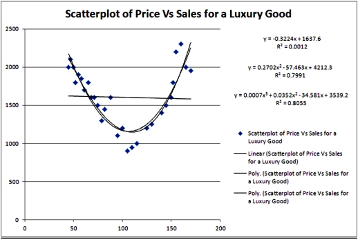 Refer to Exhibit 16.2.Using the quadratic equation,predict the sales if the luxury good is priced at $100.
A)1191.87
B)1157.64
C)1160.79
D)1168.00
Refer to Exhibit 16.2.Using the quadratic equation,predict the sales if the luxury good is priced at $100.A)1191.87
B)1157.64
C)1160.79
D)1168.00
Question
Exhibit 16-1.The following Excel scatterplot with the fitted quadratic regression equation illustrates the observed relationship between productivity and the number of hired workers. 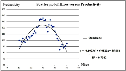 Refer to Exhibit 16.1.Predict the productivity when 32 workers are hired.
A)124.00
B)122.46
C)121.60
D)113.50
Refer to Exhibit 16.1.Predict the productivity when 32 workers are hired.A)124.00
B)122.46
C)121.60
D)113.50
Question
Exhibit 16.2.Typically,the sales volume declines with an increase of a product price.It has been observed,however,that for some luxury goods the sales volume may increase when the price increases.The following Excel output illustrates this rather unusual relationship.  Refer to Exhibit 16.2.Using the cubic regression equation,predict the sales if the luxury good is priced at $100.
A)1171.85
B)1133.10
C)1106.61
D)1092.91
Refer to Exhibit 16.2.Using the cubic regression equation,predict the sales if the luxury good is priced at $100.A)1171.85
B)1133.10
C)1106.61
D)1092.91
Question
Question
For which of the following models,the formula  = exp(b0 + b1x +
  )for finding the predicted value of y is used?
A)y = β0 + β1x + ε
B)ln(y)= β0 + β1ln(x)+ ε
C)y = β0 + β1ln(x)+ ε
D)ln(y)= β0 + β1x + ε
= exp(b0 + b1x + )for finding the predicted value of y is used?A)y = β0 + β1x + ε
B)ln(y)= β0 + β1ln(x)+ ε
C)y = β0 + β1ln(x)+ ε
D)ln(y)= β0 + β1x + ε
Question
Question
Question
Question
Question
Question
The linear and logarithmic models,y = β0 + β1x + ε and y = β0 + β1ln(x)+ ε,were used to fit given data on y and x,and the following table summarizes the regression results.Which of the two models provides a better fit? 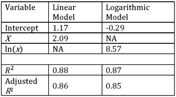
A)The linear model.
B)The logarithmic model.
C)The models are not comparable.
D)The provided information is not sufficient to make the conclusion.
A)The linear model.
B)The logarithmic model.
C)The models are not comparable.
D)The provided information is not sufficient to make the conclusion.
Question
The logarithmic and log-log models,y = β0 + β1ln(x)+ ε and ln(y)= β0 + β1ln(x)+ ε,were used to fit given data on y and x,and the following table summarizes the regression results.Which of the two models provides a better fit? 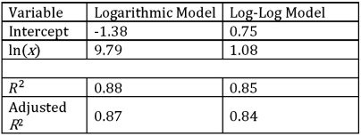
A)The logarithmic model.
B)The log-log model.
C)The models are not comparable.
D)The provided information is not sufficient to make the conclusion.
A)The logarithmic model.
B)The log-log model.
C)The models are not comparable.
D)The provided information is not sufficient to make the conclusion.
Question
Which of the regression models is most likely to provide the best fit for the data represented by the following scatterplot? 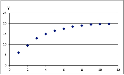
A)exponential model.
B)logarithmic model.
C)linear model.
D)log-log model.
A)exponential model.
B)logarithmic model.
C)linear model.
D)log-log model.
Question
Exhibit 16.2.Typically,the sales volume declines with an increase of a product price.It has been observed,however,that for some luxury goods the sales volume may increase when the price increases.The following Excel output illustrates this rather unusual relationship.  Refer to Exhibit 16.2.For which price do sales predicted by the quadratic equation reach their minimum?
A)106.33
B)1157.16
C)100.41
D)1166.64
Refer to Exhibit 16.2.For which price do sales predicted by the quadratic equation reach their minimum?A)106.33
B)1157.16
C)100.41
D)1166.64
Question
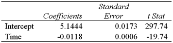
Exhibit 16-4.The following data shows the cooling temperatures of a freshly brewed cup of coffee after it is poured from the brewing pot into a serving cup.The brewing pot temperature is approximately 180º F;see http://mathbits.com/mathbits/tisection/statistics2/exponential.htm  For the assumed exponential model ln(Temp)= β0 + β1Time + ε,the following Excel regression partial output is available.
 Refer to Exhibit 16-4.What is the standard error of the estimate?
A)0.03421
B)0.45476
C)0.00177
D)0.67436
For the assumed exponential model ln(Temp)= β0 + β1Time + ε,the following Excel regression partial output is available. Refer to Exhibit 16-4.What is the standard error of the estimate?A)0.03421
B)0.45476
C)0.00177
D)0.67436
Question
For the log-log model ln(y)= β0 + β1ln(x)+ ε,the predicted value of y is computed by:
A)
B)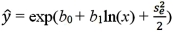
C)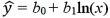
D)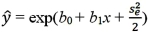
A)
B)
C)
D)
Question
Question
Exhibit 16-4.The following data shows the cooling temperatures of a freshly brewed cup of coffee after it is poured from the brewing pot into a serving cup.The brewing pot temperature is approximately 180º F;see http://mathbits.com/mathbits/tisection/statistics2/exponential.htm  For the assumed exponential model ln(Temp)= β0 + β1Time + ε,the following Excel regression partial output is available.
 Refer to Exhibit 16-4.What is the sample correlation coefficient between ln(Temp)and Time?
A)-0.9701
B)0.9701
C)-0.9849
D)0.9849
For the assumed exponential model ln(Temp)= β0 + β1Time + ε,the following Excel regression partial output is available. Refer to Exhibit 16-4.What is the sample correlation coefficient between ln(Temp)and Time?A)-0.9701
B)0.9701
C)-0.9849
D)0.9849
Question
The quadratic and logarithmic models,y = β0 + β1x + β2x2 + ε and y = β0 + β1ln(x)+ ε,were used to fit given data on y and x,and the following table summarizes the regression results.Which of the two models provides a better fit? 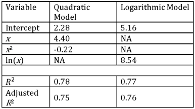
A)The quadratic model.
B)The logarithmic model.
C)The models are not comparable.
D)The provided information is not sufficient to make the conclusion.
A)The quadratic model.
B)The logarithmic model.
C)The models are not comparable.
D)The provided information is not sufficient to make the conclusion.
Question
The log-log and exponential models,ln(y)= β0 + β1ln(x)+ ε and ln(y)= β0 + β1x + ε,were used to fit given data on y and x,and the following table summarizes the regression results.Which of the two models provides a better fit? 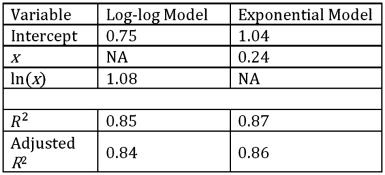
A)The log-log model.
B)The exponential model.
C)The models are not comparable.
D)The provided information is not sufficient to make the conclusion.
A)The log-log model.
B)The exponential model.
C)The models are not comparable.
D)The provided information is not sufficient to make the conclusion.
Question
Exhibit 16.2.Typically,the sales volume declines with an increase of a product price.It has been observed,however,that for some luxury goods the sales volume may increase when the price increases.The following Excel output illustrates this rather unusual relationship.  Refer to Exhibit 16.2.For which two prices are the sales predicted by the quadratic equation are 1700 units?
A)60.51 and 150.15
B)61.51 and 151.15
C)62.51 and 152.15
D)63.51 and 153.15
Refer to Exhibit 16.2.For which two prices are the sales predicted by the quadratic equation are 1700 units?A)60.51 and 150.15
B)61.51 and 151.15
C)62.51 and 152.15
D)63.51 and 153.15
Question
Exhibit 16-4.The following data shows the cooling temperatures of a freshly brewed cup of coffee after it is poured from the brewing pot into a serving cup.The brewing pot temperature is approximately 180º F;see http://mathbits.com/mathbits/tisection/statistics2/exponential.htm  For the assumed exponential model ln(Temp)= β0 + β1Time + ε,the following Excel regression partial output is available.
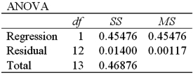
 Refer to Exhibit 16-4.What is the percentage of variations in ln(Temp)explained by Time?
A)45.48%
B)97.01%
C)1.40%
D)46.88%
For the assumed exponential model ln(Temp)= β0 + β1Time + ε,the following Excel regression partial output is available. Refer to Exhibit 16-4.What is the percentage of variations in ln(Temp)explained by Time?A)45.48%
B)97.01%
C)1.40%
D)46.88%
Question
For the logarithmic model y = β0 + β1ln(x)+ ε,the predicted value of y is computed by:
A)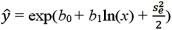
B)
C)
D)
A)
B)
C)
D)
Question
Question
Exhibit 16.6.Thirty employed single individuals were randomly selected to examine the relationship between their age (Age)and their credit card debt (Debt)expressed as a percentage of their annual income.Three polynomial models were applied and the following table summarizes Excel's regression results.  Refer to Exhibit 16.6.Using the quadratic regression equation,find the predicted maximum percentage debt.
Refer to Exhibit 16.6.Using the quadratic regression equation,find the predicted maximum percentage debt. Question
Exhibit 16.5.The following data shows the demand for an airline ticket dependent on the price of this ticket.  For the assumed cubic and log-log regression models,Demand = β0 + β1Price + β2Price2 + β3Price3 + ε and ln(Demand)= β0 + β1ln(Price)+ ε,the following regression results are available:
  Refer to Exhibit 16.5.What is the percentage of variations in ln(Demand)explained by the log-log regression equation?
A)98.52%
B)98.50%
C)91.39%
D)97.93%
For the assumed cubic and log-log regression models,Demand = β0 + β1Price + β2Price2 + β3Price3 + ε and ln(Demand)= β0 + β1ln(Price)+ ε,the following regression results are available: Refer to Exhibit 16.5.What is the percentage of variations in ln(Demand)explained by the log-log regression equation?A)98.52%
B)98.50%
C)91.39%
D)97.93%
Question
Exhibit 16.6.Thirty employed single individuals were randomly selected to examine the relationship between their age (Age)and their credit card debt (Debt)expressed as a percentage of their annual income.Three polynomial models were applied and the following table summarizes Excel's regression results.  Refer to Exhibit 16.6.Using the quadratic regression equation,find the age of an employed single person with the highest predicted percentage debt.
Refer to Exhibit 16.6.Using the quadratic regression equation,find the age of an employed single person with the highest predicted percentage debt. Question
Exhibit 16.6.Thirty employed single individuals were randomly selected to examine the relationship between their age (Age)and their credit card debt (Debt)expressed as a percentage of their annual income.Three polynomial models were applied and the following table summarizes Excel's regression results.  Refer to Exhibit 16.6.What is the sample correlation coefficient between Age and Debt?
Refer to Exhibit 16.6.What is the sample correlation coefficient between Age and Debt? Question
Exhibit 16-4.The following data shows the cooling temperatures of a freshly brewed cup of coffee after it is poured from the brewing pot into a serving cup.The brewing pot temperature is approximately 180º F;see http://mathbits.com/mathbits/tisection/statistics2/exponential.htm 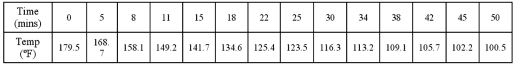 For the assumed exponential model ln(Temp)= β0 + β1Time + ε,the following Excel regression partial output is available.
 Refer to Exhibit 16-4.What is the regression equation for making predictions concerning the coffee temperature?
A)
B)
C)
D)
For the assumed exponential model ln(Temp)= β0 + β1Time + ε,the following Excel regression partial output is available. Refer to Exhibit 16-4.What is the regression equation for making predictions concerning the coffee temperature?A)
B)
C)
D)
Question
Exhibit 16-4.The following data shows the cooling temperatures of a freshly brewed cup of coffee after it is poured from the brewing pot into a serving cup.The brewing pot temperature is approximately 180º F;see http://mathbits.com/mathbits/tisection/statistics2/exponential.htm  For the assumed exponential model ln(Temp)= β0 + β1Time + ε,the following Excel regression partial output is available.
 Refer to Exhibit 16-4.How many minutes must elapse after the brewing in order to cool the coffee to 158 oF?
A)About 5 minutes
B)About 6 minutes
C)About 7 minutes
D)About 8 minutes
For the assumed exponential model ln(Temp)= β0 + β1Time + ε,the following Excel regression partial output is available. Refer to Exhibit 16-4.How many minutes must elapse after the brewing in order to cool the coffee to 158 oF?A)About 5 minutes
B)About 6 minutes
C)About 7 minutes
D)About 8 minutes
Question
Exhibit 16.5.The following data shows the demand for an airline ticket dependent on the price of this ticket.  For the assumed cubic and log-log regression models,Demand = β0 + β1Price + β2Price2 + β3Price3 + ε and ln(Demand)= β0 + β1ln(Price)+ ε,the following regression results are available:
  Refer to Exhibit 16.5.Assuming that the sample correlation coefficient between Demand and
  is 0.956,what is the percentage of variations in Demand explained by the log-log regression equation?
A)98.52%
B)98.50%
C)91.39%
D)97.93%
For the assumed cubic and log-log regression models,Demand = β0 + β1Price + β2Price2 + β3Price3 + ε and ln(Demand)= β0 + β1ln(Price)+ ε,the following regression results are available: Refer to Exhibit 16.5.Assuming that the sample correlation coefficient between Demand and is 0.956,what is the percentage of variations in Demand explained by the log-log regression equation?A)98.52%
B)98.50%
C)91.39%
D)97.93%
Question
Exhibit 16-4.The following data shows the cooling temperatures of a freshly brewed cup of coffee after it is poured from the brewing pot into a serving cup.The brewing pot temperature is approximately 180º F;see http://mathbits.com/mathbits/tisection/statistics2/exponential.htm  For the assumed exponential model ln(Temp)= β0 + β1Time + ε,the following Excel regression partial output is available.
 Refer to Exhibit 16-4.During one minute,the predicted temperature decreases by approximately
A)0.0118 0F.
B)1.18 0F.
C)1.18 %.
D)11.8 %.
For the assumed exponential model ln(Temp)= β0 + β1Time + ε,the following Excel regression partial output is available. Refer to Exhibit 16-4.During one minute,the predicted temperature decreases by approximatelyA)0.0118 0F.
B)1.18 0F.
C)1.18 %.
D)11.8 %.
Question
Exhibit 16.6.Thirty employed single individuals were randomly selected to examine the relationship between their age (Age)and their credit card debt (Debt)expressed as a percentage of their annual income.Three polynomial models were applied and the following table summarizes Excel's regression results.  Refer to Exhibit 16.6.What is the estimate of the variance of the random error ε provided by the regression equation with the best fit?
Refer to Exhibit 16.6.What is the estimate of the variance of the random error ε provided by the regression equation with the best fit? Question
Exhibit 16.5.The following data shows the demand for an airline ticket dependent on the price of this ticket. 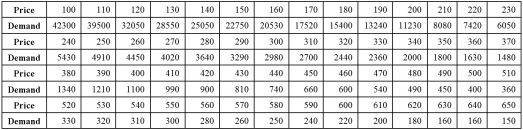 For the assumed cubic and log-log regression models,Demand = β0 + β1Price + β2Price2 + β3Price3 + ε and ln(Demand)= β0 + β1ln(Price)+ ε,the following regression results are available:
  Refer to Exhibit 16.5.Using the cubic model,what is the predicted demand when the price is $200?
A)14378.72
B)9201.45
C)10764.66
D)12499.98
For the assumed cubic and log-log regression models,Demand = β0 + β1Price + β2Price2 + β3Price3 + ε and ln(Demand)= β0 + β1ln(Price)+ ε,the following regression results are available: Refer to Exhibit 16.5.Using the cubic model,what is the predicted demand when the price is $200?A)14378.72
B)9201.45
C)10764.66
D)12499.98
Question
Exhibit 16.6.Thirty employed single individuals were randomly selected to examine the relationship between their age (Age)and their credit card debt (Debt)expressed as a percentage of their annual income.Three polynomial models were applied and the following table summarizes Excel's regression results.  Refer to Exhibit 16.6.What is the predicted percentage debt of a 45 year old employed single person determined by the model with the best fit?
Refer to Exhibit 16.6.What is the predicted percentage debt of a 45 year old employed single person determined by the model with the best fit? Question
Exhibit 16.5.The following data shows the demand for an airline ticket dependent on the price of this ticket.  For the assumed cubic and log-log regression models,Demand = β0 + β1Price + β2Price2 + β3Price3 + ε and ln(Demand)= β0 + β1ln(Price)+ ε,the following regression results are available:
  Refer to Exhibit 16.5.What does the slope of the obtained regression equation
  signify?
A)For every 1% increase in the price,the predicted demand declines by approximately 3.2577%.
B)For every 1% increase in the demand,the expected price increases by approximately 3.2577%.
C)For every 1% increase in the demand,the expected price decreases by approximately 3.2577%.
D)For every 1% increase in the price,the predicted demand increases by approximately 3.2577%.
For the assumed cubic and log-log regression models,Demand = β0 + β1Price + β2Price2 + β3Price3 + ε and ln(Demand)= β0 + β1ln(Price)+ ε,the following regression results are available: Refer to Exhibit 16.5.What does the slope of the obtained regression equation signify?A)For every 1% increase in the price,the predicted demand declines by approximately 3.2577%.
B)For every 1% increase in the demand,the expected price increases by approximately 3.2577%.
C)For every 1% increase in the demand,the expected price decreases by approximately 3.2577%.
D)For every 1% increase in the price,the predicted demand increases by approximately 3.2577%.
Question
Exhibit 16.5.The following data shows the demand for an airline ticket dependent on the price of this ticket.  For the assumed cubic and log-log regression models,Demand = β0 + β1Price + β2Price2 + β3Price3 + ε and ln(Demand)= β0 + β1ln(Price)+ ε,the following regression results are available:
  Refer to Exhibit 16.5.What is the price elasticity of the demand found by the log-log model?
A)26.3660
B)-3.2577
C)0.9852
D)0.2071
For the assumed cubic and log-log regression models,Demand = β0 + β1Price + β2Price2 + β3Price3 + ε and ln(Demand)= β0 + β1ln(Price)+ ε,the following regression results are available: Refer to Exhibit 16.5.What is the price elasticity of the demand found by the log-log model?A)26.3660
B)-3.2577
C)0.9852
D)0.2071
Question
Exhibit 16.6.Thirty employed single individuals were randomly selected to examine the relationship between their age (Age)and their credit card debt (Debt)expressed as a percentage of their annual income.Three polynomial models were applied and the following table summarizes Excel's regression results. 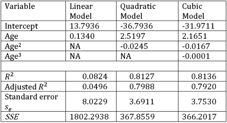 Refer to Exhibit 16.6.What is the regression equation that provides the best fit?
Refer to Exhibit 16.6.What is the regression equation that provides the best fit? Question
Exhibit 16.5.The following data shows the demand for an airline ticket dependent on the price of this ticket.  For the assumed cubic and log-log regression models,Demand = β0 + β1Price + β2Price2 + β3Price3 + ε and ln(Demand)= β0 + β1ln(Price)+ ε,the following regression results are available:
 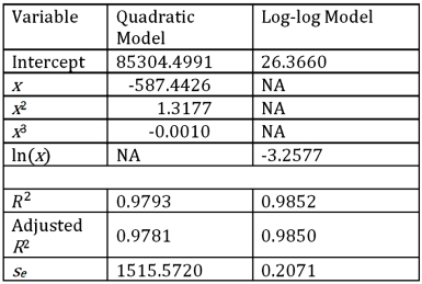 Refer to Exhibit 16.5.Using the log-log model,what is the predicted demand when the price is $200?
A)10874.92
B)9201.45
C)7849.25
D)12499.98
For the assumed cubic and log-log regression models,Demand = β0 + β1Price + β2Price2 + β3Price3 + ε and ln(Demand)= β0 + β1ln(Price)+ ε,the following regression results are available: Refer to Exhibit 16.5.Using the log-log model,what is the predicted demand when the price is $200?A)10874.92
B)9201.45
C)7849.25
D)12499.98
Question
Exhibit 16.6.Thirty employed single individuals were randomly selected to examine the relationship between their age (Age)and their credit card debt (Debt)expressed as a percentage of their annual income.Three polynomial models were applied and the following table summarizes Excel's regression results.  Refer to Exhibit 16.6.What is the value of the test statistic for testing H0: β2 = β3 = 0 against HA: β2 ≠ 0 or β3 ≠ 0 in the model Debt = β0 + β1Age + β2Age2+ β3Age3 + ε?
Refer to Exhibit 16.6.What is the value of the test statistic for testing H0: β2 = β3 = 0 against HA: β2 ≠ 0 or β3 ≠ 0 in the model Debt = β0 + β1Age + β2Age2+ β3Age3 + ε? Question
Exhibit 16.5.The following data shows the demand for an airline ticket dependent on the price of this ticket.  For the assumed cubic and log-log regression models,Demand = β0 + β1Price + β2Price2 + β3Price3 + ε and ln(Demand)= β0 + β1ln(Price)+ ε,the following regression results are available:
  Refer to Exhibit 16.5.Assuming that the sample correlation coefficient between Demand and
  is 0.956,what is the predicted demand for a price of $250 found by the model with better fit?
A)4447.88
B)3914.38
C)4029.38
D)5137.60
For the assumed cubic and log-log regression models,Demand = β0 + β1Price + β2Price2 + β3Price3 + ε and ln(Demand)= β0 + β1ln(Price)+ ε,the following regression results are available: Refer to Exhibit 16.5.Assuming that the sample correlation coefficient between Demand and is 0.956,what is the predicted demand for a price of $250 found by the model with better fit?A)4447.88
B)3914.38
C)4029.38
D)5137.60
Question
Exhibit 16.6.Thirty employed single individuals were randomly selected to examine the relationship between their age (Age)and their credit card debt (Debt)expressed as a percentage of their annual income.Three polynomial models were applied and the following table summarizes Excel's regression results.  Refer to Exhibit 16.6.What is the percentage of variations in Debt explained by Age in the regression equation with the best fit?
Refer to Exhibit 16.6.What is the percentage of variations in Debt explained by Age in the regression equation with the best fit? Question
Exhibit 16-4.The following data shows the cooling temperatures of a freshly brewed cup of coffee after it is poured from the brewing pot into a serving cup.The brewing pot temperature is approximately 180º F;see http://mathbits.com/mathbits/tisection/statistics2/exponential.htm  For the assumed exponential model ln(Temp)= β0 + β1Time + ε,the following Excel regression partial output is available.
 Refer to Exhibit 16-4.What is the predicted coffee temperature in half an hour after the brewing?
A)164.72
B)-4.7904
C)164.74
D)120.42
For the assumed exponential model ln(Temp)= β0 + β1Time + ε,the following Excel regression partial output is available. Refer to Exhibit 16-4.What is the predicted coffee temperature in half an hour after the brewing?A)164.72
B)-4.7904
C)164.74
D)120.42
Question
Exhibit 16.6.Thirty employed single individuals were randomly selected to examine the relationship between their age (Age)and their credit card debt (Debt)expressed as a percentage of their annual income.Three polynomial models were applied and the following table summarizes Excel's regression results.  Refer to Exhibit 16.6.If you impose the restrictions β2 = β3 = 0 on the model Debt = β0 + β1Age + β2Age2+ β3Age3 + ε,what will be the sum of the squared errors (SSER)computed for the restricted model?
Refer to Exhibit 16.6.If you impose the restrictions β2 = β3 = 0 on the model Debt = β0 + β1Age + β2Age2+ β3Age3 + ε,what will be the sum of the squared errors (SSER)computed for the restricted model?
Unlock Deck
Sign up to unlock the cards in this deck!
Unlock Deck
Unlock Deck
1/95
Play
Full screen (f)
Deck 16: Regression Models for Nonlinear Relationships
1
The regression model ln(y)= β0 + β1x + ε is called exponential.
True
2
Many non-linear regression models can be studied under the linear regression framework using transformation of the response variable and/or the explanatory variables.
True
3
If the data is available on the response variable y and the explanatory variable x,and the fit of the quadratic model y = β0 + β1x + β2x2 + ε is to be tested,standard linear regression can be applied on:
A)y and x
B)y,x and x2
C)y,xy,and x2
D)y,y2 and x2
A)y and x
B)y,x and x2
C)y,xy,and x2
D)y,y2 and x2
y,x and x2
4
Although a polynomial regression model of order two or more is nonlinear,when it is fitted to the data we use the _______ regression to make this fit.
A)nonlinear
B)logistic
C)polynomial
D)linear
A)nonlinear
B)logistic
C)polynomial
D)linear
Unlock Deck
Unlock for access to all 95 flashcards in this deck.
Unlock Deck
k this deck
5
For the logarithmic model y = β0 + β1ln(x)+ ε,β1/100 is the approximate change in E(y)when x increases by one percent.
Unlock Deck
Unlock for access to all 95 flashcards in this deck.
Unlock Deck
k this deck
6
The fit of the models y = β0 + β1x + ε and ln(y)= β0 + β1x + ε can be compared using the coefficients R2 found in the two corresponding Excel's regression outputs.
Unlock Deck
Unlock for access to all 95 flashcards in this deck.
Unlock Deck
k this deck
7
The fit of the regression equations and can be compared using the coefficient of determination R2.
and can be compared using the coefficient of determination R2. Unlock Deck
Unlock for access to all 95 flashcards in this deck.
Unlock Deck
k this deck
8
When the data is available on x and y,it is easy to estimate a polynomial regression model.
Unlock Deck
Unlock for access to all 95 flashcards in this deck.
Unlock Deck
k this deck
9
For the exponential model ln(y)= β0 + β1x + ε,β1 × 100% is the approximate percentage change in E(y)when x increases by one percent.
Unlock Deck
Unlock for access to all 95 flashcards in this deck.
Unlock Deck
k this deck
10
How many coefficients have to be estimated in the quadratic regression modely = β0 + β1x + β2x2 + ε?
A)4
B)3
C)2
D)1
A)4
B)3
C)2
D)1
Unlock Deck
Unlock for access to all 95 flashcards in this deck.
Unlock Deck
k this deck
11
The fit of the models y = β0 + β1x + β2x2 + ε and y = β0 + β1ln(x)+ ε can be compared using the coefficient of determination R2.
Unlock Deck
Unlock for access to all 95 flashcards in this deck.
Unlock Deck
k this deck
12
A quadratic regression model is a special type of a polynomial regression model.
Unlock Deck
Unlock for access to all 95 flashcards in this deck.
Unlock Deck
k this deck
13
The fit of the models y = β0 + β1x + ε and y = β0 + β1ln(x)+ ε can be compared using the coefficient of determination R2.
Unlock Deck
Unlock for access to all 95 flashcards in this deck.
Unlock Deck
k this deck
14
Which of the following is a quadratic regression equation?
A)
B)
C)
D)
A)
B)
C)
D)
Unlock Deck
Unlock for access to all 95 flashcards in this deck.
Unlock Deck
k this deck
15
The curve representing the regression equation has a U-shape if b2 > 0.
has a U-shape if b2 > 0. Unlock Deck
Unlock for access to all 95 flashcards in this deck.
Unlock Deck
k this deck
16
The cubic regression model,y = β0 + β1x + β2x2+ β3x3 + ε,is used when we assume that the relationship between x and y should be captured by a function that has either minimum or maximum,but not both.
Unlock Deck
Unlock for access to all 95 flashcards in this deck.
Unlock Deck
k this deck
17
Which of the following regression models is not polynomial?
A)y = β0 + β1x + ε
B)y = β0 + β1x + β2x2 + ε
C)y = β0 + β1x-1 + ε
D)y = β0 + β1x + β2x2+ β3x3 + ε
A)y = β0 + β1x + ε
B)y = β0 + β1x + β2x2 + ε
C)y = β0 + β1x-1 + ε
D)y = β0 + β1x + β2x2+ β3x3 + ε
Unlock Deck
Unlock for access to all 95 flashcards in this deck.
Unlock Deck
k this deck
18
The equation y = β0 + β1x + β2x2 + ε is called a cubic regression model.
Unlock Deck
Unlock for access to all 95 flashcards in this deck.
Unlock Deck
k this deck
19
The regression model ln(y)= β0 + β1ln(x)+ ε is called logarithmic.
Unlock Deck
Unlock for access to all 95 flashcards in this deck.
Unlock Deck
k this deck
20
For the model ln(y)= β0 + β1ln(x)+ ε with 0 < β1 < 1,if x increases than E(y)increases but at a slower rate.
Unlock Deck
Unlock for access to all 95 flashcards in this deck.
Unlock Deck
k this deck
21
Exhibit 16-1.The following Excel scatterplot with the fitted quadratic regression equation illustrates the observed relationship between productivity and the number of hired workers. Refer to Exhibit 16.1.For which value of Hires the predicted Productivity is maximized (Do not round to the nearest integer. )?
A)29.58
B)124.60
C)35.086
D)27.34
Refer to Exhibit 16.1.For which value of Hires the predicted Productivity is maximized (Do not round to the nearest integer. )?A)29.58
B)124.60
C)35.086
D)27.34
Unlock Deck
Unlock for access to all 95 flashcards in this deck.
Unlock Deck
k this deck
22
What is the effect of b2 < 0 in the case of the quadratic equation ?
A)The curve is U-shaped.
B)The curve is inverted U-shaped.
C)The curve is a straight line.
D)The curve is not a parabola.
?A)The curve is U-shaped.
B)The curve is inverted U-shaped.
C)The curve is a straight line.
D)The curve is not a parabola.
Unlock Deck
Unlock for access to all 95 flashcards in this deck.
Unlock Deck
k this deck
23
Exhibit 16.2.Typically,the sales volume declines with an increase of a product price.It has been observed,however,that for some luxury goods the sales volume may increase when the price increases.The following Excel output illustrates this rather unusual relationship. Refer to Exhibit 16.2.For the considered range of the price,the relationship between Price and Sales should be described by a:
A)concave function.
B)hyperbola.
C)convex function.
D)linear function.
Refer to Exhibit 16.2.For the considered range of the price,the relationship between Price and Sales should be described by a:A)concave function.
B)hyperbola.
C)convex function.
D)linear function.
Unlock Deck
Unlock for access to all 95 flashcards in this deck.
Unlock Deck
k this deck
24
Exhibit 16-1.The following Excel scatterplot with the fitted quadratic regression equation illustrates the observed relationship between productivity and the number of hired workers. Refer to Exhibit 16.1.Assuming that the values of Hires can be non-integers,what is the maximum value of Productivity?
A)29.58
B)124.603
C)35.086
D)127.50
Refer to Exhibit 16.1.Assuming that the values of Hires can be non-integers,what is the maximum value of Productivity?A)29.58
B)124.603
C)35.086
D)127.50
Unlock Deck
Unlock for access to all 95 flashcards in this deck.
Unlock Deck
k this deck
25
For the quadratic regression equation ,the predicted y achieves its optimum (maximum or minimum)when x is:
A)
B)
C)
D)
,the predicted y achieves its optimum (maximum or minimum)when x is:A)
B)
C)
D)
Unlock Deck
Unlock for access to all 95 flashcards in this deck.
Unlock Deck
k this deck
26
An inverted U-shaped curve is also known to be:
A)concave
B)convex
C)opaque
D)hyperbola
A)concave
B)convex
C)opaque
D)hyperbola
Unlock Deck
Unlock for access to all 95 flashcards in this deck.
Unlock Deck
k this deck
27
Exhibit 16-1.The following Excel scatterplot with the fitted quadratic regression equation illustrates the observed relationship between productivity and the number of hired workers. Refer to Exhibit 16.1.The quadratic regression equation found is:
A) = 35.086 + 6.0523Hires - 0.1023Hires2.
B) = 6.0523 + 35.086Hires - 0.1023Hires2.
C) = 6.0523 - 35.086Hires + 0.1023Hires2.
D)
Refer to Exhibit 16.1.The quadratic regression equation found is:A)
= 35.086 + 6.0523Hires - 0.1023Hires2.B)
= 6.0523 + 35.086Hires - 0.1023Hires2.C)
= 6.0523 - 35.086Hires + 0.1023Hires2.D)
Unlock Deck
Unlock for access to all 95 flashcards in this deck.
Unlock Deck
k this deck
28
Exhibit 16-1.The following Excel scatterplot with the fitted quadratic regression equation illustrates the observed relationship between productivity and the number of hired workers. Refer to Exhibit 16.1.What is the percentage of variations in the productivity explained by the number of hired workers?
A)85.69%
B)0.7342%
C)90.54%
D)73.42%
Refer to Exhibit 16.1.What is the percentage of variations in the productivity explained by the number of hired workers?A)85.69%
B)0.7342%
C)90.54%
D)73.42%
Unlock Deck
Unlock for access to all 95 flashcards in this deck.
Unlock Deck
k this deck
29
For the quadratic regression equation ,the optimum (maximum or minimum)value of is:
A)
B)
C)
D)
,the optimum (maximum or minimum)value of is:A)
B)
C)
D)
Unlock Deck
Unlock for access to all 95 flashcards in this deck.
Unlock Deck
k this deck
30
Exhibit 16.2.Typically,the sales volume declines with an increase of a product price.It has been observed,however,that for some luxury goods the sales volume may increase when the price increases.The following Excel output illustrates this rather unusual relationship. Refer to Exhibit 16.2.What can be said about the linear relationship between Price and Sales?
A)The relationship is negatively moderate.
B)There is no relationship.
C)The relationship is positively strong.
D)The relationship is negatively strong.
Refer to Exhibit 16.2.What can be said about the linear relationship between Price and Sales?A)The relationship is negatively moderate.
B)There is no relationship.
C)The relationship is positively strong.
D)The relationship is negatively strong.
Unlock Deck
Unlock for access to all 95 flashcards in this deck.
Unlock Deck
k this deck
31
Exhibit 16-1.The following Excel scatterplot with the fitted quadratic regression equation illustrates the observed relationship between productivity and the number of hired workers. Refer to Exhibit 16.1.Assuming that the number of hired workers must be integer,what is the maximum productivity to achieve?
A)29.58
B)30.00
C)124.603
D)124.585
Refer to Exhibit 16.1.Assuming that the number of hired workers must be integer,what is the maximum productivity to achieve?A)29.58
B)30.00
C)124.603
D)124.585
Unlock Deck
Unlock for access to all 95 flashcards in this deck.
Unlock Deck
k this deck
32
Given the data on y and x,what is needed to run Excel regression for the polynomial model of order 3?
A)Creating the values of one pseudo-explanatory variable by squaring the values of x.
B)Creating the values of two pseudo-explanatory variables by squaring and cubing the values of x,respectively.
C)Creating the values of three pseudo-explanatory variables by raising the values of x to the power of 2,3 and 4,respectively.
D)Nothing is needeD.
A)Creating the values of one pseudo-explanatory variable by squaring the values of x.
B)Creating the values of two pseudo-explanatory variables by squaring and cubing the values of x,respectively.
C)Creating the values of three pseudo-explanatory variables by raising the values of x to the power of 2,3 and 4,respectively.
D)Nothing is needeD.
Unlock Deck
Unlock for access to all 95 flashcards in this deck.
Unlock Deck
k this deck
33
Exhibit 16-1.The following Excel scatterplot with the fitted quadratic regression equation illustrates the observed relationship between productivity and the number of hired workers. Refer to Exhibit 16.1.Assuming that the number of hired workers must be integer,how many workers should be hired in order to achieve the highest productivity?
A)26
B)28
C)30
D)32
Refer to Exhibit 16.1.Assuming that the number of hired workers must be integer,how many workers should be hired in order to achieve the highest productivity?A)26
B)28
C)30
D)32
Unlock Deck
Unlock for access to all 95 flashcards in this deck.
Unlock Deck
k this deck
34
Exhibit 16.2.Typically,the sales volume declines with an increase of a product price.It has been observed,however,that for some luxury goods the sales volume may increase when the price increases.The following Excel output illustrates this rather unusual relationship. Refer to Exhibit 16.2.What is the number of estimated coefficients of the cubic regression model?
A)1
B)2
C)3
D)4
Refer to Exhibit 16.2.What is the number of estimated coefficients of the cubic regression model?A)1
B)2
C)3
D)4
Unlock Deck
Unlock for access to all 95 flashcards in this deck.
Unlock Deck
k this deck
35
For the quadratic equation ,which of the following expressions must be zero in order to minimize or maximize the predicted y?
A)b1 + 2b2x
B)2b1 + b2x
C)
D)
,which of the following expressions must be zero in order to minimize or maximize the predicted y?A)b1 + 2b2x
B)2b1 + b2x
C)
D)
Unlock Deck
Unlock for access to all 95 flashcards in this deck.
Unlock Deck
k this deck
36
Exhibit 16.2.Typically,the sales volume declines with an increase of a product price.It has been observed,however,that for some luxury goods the sales volume may increase when the price increases.The following Excel output illustrates this rather unusual relationship. Refer to Exhibit 16.2.Which of the following models is most likely to be chosen in order to describe the relationship between Price and Sales?
A)Linear
B)Quadratic
C)Cubic
D)Exponential
Refer to Exhibit 16.2.Which of the following models is most likely to be chosen in order to describe the relationship between Price and Sales?A)Linear
B)Quadratic
C)Cubic
D)Exponential
Unlock Deck
Unlock for access to all 95 flashcards in this deck.
Unlock Deck
k this deck
37
Exhibit 16.2.Typically,the sales volume declines with an increase of a product price.It has been observed,however,that for some luxury goods the sales volume may increase when the price increases.The following Excel output illustrates this rather unusual relationship. Refer to Exhibit 16.2.Using the quadratic equation,predict the sales if the luxury good is priced at $100.
A)1191.87
B)1157.64
C)1160.79
D)1168.00
Refer to Exhibit 16.2.Using the quadratic equation,predict the sales if the luxury good is priced at $100.A)1191.87
B)1157.64
C)1160.79
D)1168.00
Unlock Deck
Unlock for access to all 95 flashcards in this deck.
Unlock Deck
k this deck
38
Exhibit 16-1.The following Excel scatterplot with the fitted quadratic regression equation illustrates the observed relationship between productivity and the number of hired workers. Refer to Exhibit 16.1.Predict the productivity when 32 workers are hired.
A)124.00
B)122.46
C)121.60
D)113.50
Refer to Exhibit 16.1.Predict the productivity when 32 workers are hired.A)124.00
B)122.46
C)121.60
D)113.50
Unlock Deck
Unlock for access to all 95 flashcards in this deck.
Unlock Deck
k this deck
39
Exhibit 16.2.Typically,the sales volume declines with an increase of a product price.It has been observed,however,that for some luxury goods the sales volume may increase when the price increases.The following Excel output illustrates this rather unusual relationship. Refer to Exhibit 16.2.Using the cubic regression equation,predict the sales if the luxury good is priced at $100.
A)1171.85
B)1133.10
C)1106.61
D)1092.91
Refer to Exhibit 16.2.Using the cubic regression equation,predict the sales if the luxury good is priced at $100.A)1171.85
B)1133.10
C)1106.61
D)1092.91
Unlock Deck
Unlock for access to all 95 flashcards in this deck.
Unlock Deck
k this deck
40
The coefficient of determination R2 cannot be used to compare the linear and quadratic models,because:
A)the quadratic model has one parameter more to estimate.
B)the quadratic model has two parameters more to estimate.
C)the quadratic model always has a lower R2.
D)R2 is not defined for the quadratic model.
A)the quadratic model has one parameter more to estimate.
B)the quadratic model has two parameters more to estimate.
C)the quadratic model always has a lower R2.
D)R2 is not defined for the quadratic model.
Unlock Deck
Unlock for access to all 95 flashcards in this deck.
Unlock Deck
k this deck
41
For which of the following models,the formula = exp(b0 + b1x + )for finding the predicted value of y is used?
A)y = β0 + β1x + ε
B)ln(y)= β0 + β1ln(x)+ ε
C)y = β0 + β1ln(x)+ ε
D)ln(y)= β0 + β1x + ε
= exp(b0 + b1x + )for finding the predicted value of y is used?A)y = β0 + β1x + ε
B)ln(y)= β0 + β1ln(x)+ ε
C)y = β0 + β1ln(x)+ ε
D)ln(y)= β0 + β1x + ε
Unlock Deck
Unlock for access to all 95 flashcards in this deck.
Unlock Deck
k this deck
42
A model in which the response variable is transformed into its natural logarithm is called a(n)_____.
A)log-log model
B)logarithmic model
C)exponential model
D)linear model
A)log-log model
B)logarithmic model
C)exponential model
D)linear model
Unlock Deck
Unlock for access to all 95 flashcards in this deck.
Unlock Deck
k this deck
43
When the predicted value of the response variable has to be found,in which of the following two models,is there a need for the standard error correction?
A)Linear and Log-log
B)Log-log and Logarithmic
C)Logarithmic and Linear
D)Log-log and Exponential
A)Linear and Log-log
B)Log-log and Logarithmic
C)Logarithmic and Linear
D)Log-log and Exponential
Unlock Deck
Unlock for access to all 95 flashcards in this deck.
Unlock Deck
k this deck
44
In the model ln(y)= β0 + β1ln(x)+ ε,the coefficient β1 is the approximate:
A)change in E(y)when x increases by one unit.
B)percentage change in E(y)when x increases by 1%.
C)percentage change in E(y)when x increases by one unit.
D)change in E(y)when x increases by 1%.
A)change in E(y)when x increases by one unit.
B)percentage change in E(y)when x increases by 1%.
C)percentage change in E(y)when x increases by one unit.
D)change in E(y)when x increases by 1%.
Unlock Deck
Unlock for access to all 95 flashcards in this deck.
Unlock Deck
k this deck
45
A model with one explanatory variable being the only one transformed into its natural logarithm is called a(n)_____.
A)log-log model
B)logarithmic model
C)exponential model
D)linear model
A)log-log model
B)logarithmic model
C)exponential model
D)linear model
Unlock Deck
Unlock for access to all 95 flashcards in this deck.
Unlock Deck
k this deck
46
For the exponential model ln(y)= β0 + β1x + ε,if x increases by 1 unit,then E(y)changes by approximately
A)β1 × 100 percent.
B)β1 × 100 units.
C)β1 percent.
D)β1 units.
A)β1 × 100 percent.
B)β1 × 100 units.
C)β1 percent.
D)β1 units.
Unlock Deck
Unlock for access to all 95 flashcards in this deck.
Unlock Deck
k this deck
47
The linear and logarithmic models,y = β0 + β1x + ε and y = β0 + β1ln(x)+ ε,were used to fit given data on y and x,and the following table summarizes the regression results.Which of the two models provides a better fit?
A)The linear model.
B)The logarithmic model.
C)The models are not comparable.
D)The provided information is not sufficient to make the conclusion.
A)The linear model.
B)The logarithmic model.
C)The models are not comparable.
D)The provided information is not sufficient to make the conclusion.
Unlock Deck
Unlock for access to all 95 flashcards in this deck.
Unlock Deck
k this deck
48
The logarithmic and log-log models,y = β0 + β1ln(x)+ ε and ln(y)= β0 + β1ln(x)+ ε,were used to fit given data on y and x,and the following table summarizes the regression results.Which of the two models provides a better fit?
A)The logarithmic model.
B)The log-log model.
C)The models are not comparable.
D)The provided information is not sufficient to make the conclusion.
A)The logarithmic model.
B)The log-log model.
C)The models are not comparable.
D)The provided information is not sufficient to make the conclusion.
Unlock Deck
Unlock for access to all 95 flashcards in this deck.
Unlock Deck
k this deck
49
Which of the regression models is most likely to provide the best fit for the data represented by the following scatterplot?
A)exponential model.
B)logarithmic model.
C)linear model.
D)log-log model.
A)exponential model.
B)logarithmic model.
C)linear model.
D)log-log model.
Unlock Deck
Unlock for access to all 95 flashcards in this deck.
Unlock Deck
k this deck
50
Exhibit 16.2.Typically,the sales volume declines with an increase of a product price.It has been observed,however,that for some luxury goods the sales volume may increase when the price increases.The following Excel output illustrates this rather unusual relationship. Refer to Exhibit 16.2.For which price do sales predicted by the quadratic equation reach their minimum?
A)106.33
B)1157.16
C)100.41
D)1166.64
Refer to Exhibit 16.2.For which price do sales predicted by the quadratic equation reach their minimum?A)106.33
B)1157.16
C)100.41
D)1166.64
Unlock Deck
Unlock for access to all 95 flashcards in this deck.
Unlock Deck
k this deck
51
Exhibit 16-4.The following data shows the cooling temperatures of a freshly brewed cup of coffee after it is poured from the brewing pot into a serving cup.The brewing pot temperature is approximately 180º F;see http://mathbits.com/mathbits/tisection/statistics2/exponential.htm For the assumed exponential model ln(Temp)= β0 + β1Time + ε,the following Excel regression partial output is available. Refer to Exhibit 16-4.What is the standard error of the estimate?
A)0.03421
B)0.45476
C)0.00177
D)0.67436
For the assumed exponential model ln(Temp)= β0 + β1Time + ε,the following Excel regression partial output is available. Refer to Exhibit 16-4.What is the standard error of the estimate?A)0.03421
B)0.45476
C)0.00177
D)0.67436
Unlock Deck
Unlock for access to all 95 flashcards in this deck.
Unlock Deck
k this deck
52
For the log-log model ln(y)= β0 + β1ln(x)+ ε,the predicted value of y is computed by:
A)
B)
C)
D)
A)
B)
C)
D)
Unlock Deck
Unlock for access to all 95 flashcards in this deck.
Unlock Deck
k this deck
53
A model in which both the response variable and the explanatory variable are transformed into their natural logarithms is better known as a(n):
A)exponential model.
B)logarithmic model.
C)linear model.
D)log-log model.
A)exponential model.
B)logarithmic model.
C)linear model.
D)log-log model.
Unlock Deck
Unlock for access to all 95 flashcards in this deck.
Unlock Deck
k this deck
54
Exhibit 16-4.The following data shows the cooling temperatures of a freshly brewed cup of coffee after it is poured from the brewing pot into a serving cup.The brewing pot temperature is approximately 180º F;see http://mathbits.com/mathbits/tisection/statistics2/exponential.htm For the assumed exponential model ln(Temp)= β0 + β1Time + ε,the following Excel regression partial output is available. Refer to Exhibit 16-4.What is the sample correlation coefficient between ln(Temp)and Time?
A)-0.9701
B)0.9701
C)-0.9849
D)0.9849
For the assumed exponential model ln(Temp)= β0 + β1Time + ε,the following Excel regression partial output is available. Refer to Exhibit 16-4.What is the sample correlation coefficient between ln(Temp)and Time?A)-0.9701
B)0.9701
C)-0.9849
D)0.9849
Unlock Deck
Unlock for access to all 95 flashcards in this deck.
Unlock Deck
k this deck
55
The quadratic and logarithmic models,y = β0 + β1x + β2x2 + ε and y = β0 + β1ln(x)+ ε,were used to fit given data on y and x,and the following table summarizes the regression results.Which of the two models provides a better fit?
A)The quadratic model.
B)The logarithmic model.
C)The models are not comparable.
D)The provided information is not sufficient to make the conclusion.
A)The quadratic model.
B)The logarithmic model.
C)The models are not comparable.
D)The provided information is not sufficient to make the conclusion.
Unlock Deck
Unlock for access to all 95 flashcards in this deck.
Unlock Deck
k this deck
56
The log-log and exponential models,ln(y)= β0 + β1ln(x)+ ε and ln(y)= β0 + β1x + ε,were used to fit given data on y and x,and the following table summarizes the regression results.Which of the two models provides a better fit?
A)The log-log model.
B)The exponential model.
C)The models are not comparable.
D)The provided information is not sufficient to make the conclusion.
A)The log-log model.
B)The exponential model.
C)The models are not comparable.
D)The provided information is not sufficient to make the conclusion.
Unlock Deck
Unlock for access to all 95 flashcards in this deck.
Unlock Deck
k this deck
57
Exhibit 16.2.Typically,the sales volume declines with an increase of a product price.It has been observed,however,that for some luxury goods the sales volume may increase when the price increases.The following Excel output illustrates this rather unusual relationship. Refer to Exhibit 16.2.For which two prices are the sales predicted by the quadratic equation are 1700 units?
A)60.51 and 150.15
B)61.51 and 151.15
C)62.51 and 152.15
D)63.51 and 153.15
Refer to Exhibit 16.2.For which two prices are the sales predicted by the quadratic equation are 1700 units?A)60.51 and 150.15
B)61.51 and 151.15
C)62.51 and 152.15
D)63.51 and 153.15
Unlock Deck
Unlock for access to all 95 flashcards in this deck.
Unlock Deck
k this deck
58
Exhibit 16-4.The following data shows the cooling temperatures of a freshly brewed cup of coffee after it is poured from the brewing pot into a serving cup.The brewing pot temperature is approximately 180º F;see http://mathbits.com/mathbits/tisection/statistics2/exponential.htm For the assumed exponential model ln(Temp)= β0 + β1Time + ε,the following Excel regression partial output is available. Refer to Exhibit 16-4.What is the percentage of variations in ln(Temp)explained by Time?
A)45.48%
B)97.01%
C)1.40%
D)46.88%
For the assumed exponential model ln(Temp)= β0 + β1Time + ε,the following Excel regression partial output is available. Refer to Exhibit 16-4.What is the percentage of variations in ln(Temp)explained by Time?A)45.48%
B)97.01%
C)1.40%
D)46.88%
Unlock Deck
Unlock for access to all 95 flashcards in this deck.
Unlock Deck
k this deck
59
For the logarithmic model y = β0 + β1ln(x)+ ε,the predicted value of y is computed by:
A)
B)
C)
D)
A)
B)
C)
D)
Unlock Deck
Unlock for access to all 95 flashcards in this deck.
Unlock Deck
k this deck
60
What does a positive value for price elasticity indicate if y represents the quantity demanded of a particular good and x is its unit price in a log-log regression model?
A)As price increases,the expected sales decreases.
B)As price decreases,the expected sales increases.
C)As price increases,the expected sales increases.
D)As price decreases,the expected sales remain the same.
A)As price increases,the expected sales decreases.
B)As price decreases,the expected sales increases.
C)As price increases,the expected sales increases.
D)As price decreases,the expected sales remain the same.
Unlock Deck
Unlock for access to all 95 flashcards in this deck.
Unlock Deck
k this deck
61
Exhibit 16.6.Thirty employed single individuals were randomly selected to examine the relationship between their age (Age)and their credit card debt (Debt)expressed as a percentage of their annual income.Three polynomial models were applied and the following table summarizes Excel's regression results. Refer to Exhibit 16.6.Using the quadratic regression equation,find the predicted maximum percentage debt.
Refer to Exhibit 16.6.Using the quadratic regression equation,find the predicted maximum percentage debt. Unlock Deck
Unlock for access to all 95 flashcards in this deck.
Unlock Deck
k this deck
62
Exhibit 16.5.The following data shows the demand for an airline ticket dependent on the price of this ticket. For the assumed cubic and log-log regression models,Demand = β0 + β1Price + β2Price2 + β3Price3 + ε and ln(Demand)= β0 + β1ln(Price)+ ε,the following regression results are available: Refer to Exhibit 16.5.What is the percentage of variations in ln(Demand)explained by the log-log regression equation?
A)98.52%
B)98.50%
C)91.39%
D)97.93%
For the assumed cubic and log-log regression models,Demand = β0 + β1Price + β2Price2 + β3Price3 + ε and ln(Demand)= β0 + β1ln(Price)+ ε,the following regression results are available: Refer to Exhibit 16.5.What is the percentage of variations in ln(Demand)explained by the log-log regression equation?A)98.52%
B)98.50%
C)91.39%
D)97.93%
Unlock Deck
Unlock for access to all 95 flashcards in this deck.
Unlock Deck
k this deck
63
Exhibit 16.6.Thirty employed single individuals were randomly selected to examine the relationship between their age (Age)and their credit card debt (Debt)expressed as a percentage of their annual income.Three polynomial models were applied and the following table summarizes Excel's regression results. Refer to Exhibit 16.6.Using the quadratic regression equation,find the age of an employed single person with the highest predicted percentage debt.
Refer to Exhibit 16.6.Using the quadratic regression equation,find the age of an employed single person with the highest predicted percentage debt. Unlock Deck
Unlock for access to all 95 flashcards in this deck.
Unlock Deck
k this deck
64
Exhibit 16.6.Thirty employed single individuals were randomly selected to examine the relationship between their age (Age)and their credit card debt (Debt)expressed as a percentage of their annual income.Three polynomial models were applied and the following table summarizes Excel's regression results. Refer to Exhibit 16.6.What is the sample correlation coefficient between Age and Debt?
Refer to Exhibit 16.6.What is the sample correlation coefficient between Age and Debt? Unlock Deck
Unlock for access to all 95 flashcards in this deck.
Unlock Deck
k this deck
65
Exhibit 16-4.The following data shows the cooling temperatures of a freshly brewed cup of coffee after it is poured from the brewing pot into a serving cup.The brewing pot temperature is approximately 180º F;see http://mathbits.com/mathbits/tisection/statistics2/exponential.htm For the assumed exponential model ln(Temp)= β0 + β1Time + ε,the following Excel regression partial output is available. Refer to Exhibit 16-4.What is the regression equation for making predictions concerning the coffee temperature?
A)
B)
C)
D)
For the assumed exponential model ln(Temp)= β0 + β1Time + ε,the following Excel regression partial output is available. Refer to Exhibit 16-4.What is the regression equation for making predictions concerning the coffee temperature?A)
B)
C)
D)
Unlock Deck
Unlock for access to all 95 flashcards in this deck.
Unlock Deck
k this deck
66
Exhibit 16-4.The following data shows the cooling temperatures of a freshly brewed cup of coffee after it is poured from the brewing pot into a serving cup.The brewing pot temperature is approximately 180º F;see http://mathbits.com/mathbits/tisection/statistics2/exponential.htm For the assumed exponential model ln(Temp)= β0 + β1Time + ε,the following Excel regression partial output is available. Refer to Exhibit 16-4.How many minutes must elapse after the brewing in order to cool the coffee to 158 oF?
A)About 5 minutes
B)About 6 minutes
C)About 7 minutes
D)About 8 minutes
For the assumed exponential model ln(Temp)= β0 + β1Time + ε,the following Excel regression partial output is available. Refer to Exhibit 16-4.How many minutes must elapse after the brewing in order to cool the coffee to 158 oF?A)About 5 minutes
B)About 6 minutes
C)About 7 minutes
D)About 8 minutes
Unlock Deck
Unlock for access to all 95 flashcards in this deck.
Unlock Deck
k this deck
67
Exhibit 16.5.The following data shows the demand for an airline ticket dependent on the price of this ticket. For the assumed cubic and log-log regression models,Demand = β0 + β1Price + β2Price2 + β3Price3 + ε and ln(Demand)= β0 + β1ln(Price)+ ε,the following regression results are available: Refer to Exhibit 16.5.Assuming that the sample correlation coefficient between Demand and is 0.956,what is the percentage of variations in Demand explained by the log-log regression equation?
A)98.52%
B)98.50%
C)91.39%
D)97.93%
For the assumed cubic and log-log regression models,Demand = β0 + β1Price + β2Price2 + β3Price3 + ε and ln(Demand)= β0 + β1ln(Price)+ ε,the following regression results are available: Refer to Exhibit 16.5.Assuming that the sample correlation coefficient between Demand and is 0.956,what is the percentage of variations in Demand explained by the log-log regression equation?A)98.52%
B)98.50%
C)91.39%
D)97.93%
Unlock Deck
Unlock for access to all 95 flashcards in this deck.
Unlock Deck
k this deck
68
Exhibit 16-4.The following data shows the cooling temperatures of a freshly brewed cup of coffee after it is poured from the brewing pot into a serving cup.The brewing pot temperature is approximately 180º F;see http://mathbits.com/mathbits/tisection/statistics2/exponential.htm For the assumed exponential model ln(Temp)= β0 + β1Time + ε,the following Excel regression partial output is available. Refer to Exhibit 16-4.During one minute,the predicted temperature decreases by approximately
A)0.0118 0F.
B)1.18 0F.
C)1.18 %.
D)11.8 %.
For the assumed exponential model ln(Temp)= β0 + β1Time + ε,the following Excel regression partial output is available. Refer to Exhibit 16-4.During one minute,the predicted temperature decreases by approximatelyA)0.0118 0F.
B)1.18 0F.
C)1.18 %.
D)11.8 %.
Unlock Deck
Unlock for access to all 95 flashcards in this deck.
Unlock Deck
k this deck
69
Exhibit 16.6.Thirty employed single individuals were randomly selected to examine the relationship between their age (Age)and their credit card debt (Debt)expressed as a percentage of their annual income.Three polynomial models were applied and the following table summarizes Excel's regression results. Refer to Exhibit 16.6.What is the estimate of the variance of the random error ε provided by the regression equation with the best fit?
Refer to Exhibit 16.6.What is the estimate of the variance of the random error ε provided by the regression equation with the best fit? Unlock Deck
Unlock for access to all 95 flashcards in this deck.
Unlock Deck
k this deck
70
Exhibit 16.5.The following data shows the demand for an airline ticket dependent on the price of this ticket. For the assumed cubic and log-log regression models,Demand = β0 + β1Price + β2Price2 + β3Price3 + ε and ln(Demand)= β0 + β1ln(Price)+ ε,the following regression results are available: Refer to Exhibit 16.5.Using the cubic model,what is the predicted demand when the price is $200?
A)14378.72
B)9201.45
C)10764.66
D)12499.98
For the assumed cubic and log-log regression models,Demand = β0 + β1Price + β2Price2 + β3Price3 + ε and ln(Demand)= β0 + β1ln(Price)+ ε,the following regression results are available: Refer to Exhibit 16.5.Using the cubic model,what is the predicted demand when the price is $200?A)14378.72
B)9201.45
C)10764.66
D)12499.98
Unlock Deck
Unlock for access to all 95 flashcards in this deck.
Unlock Deck
k this deck
71
Exhibit 16.6.Thirty employed single individuals were randomly selected to examine the relationship between their age (Age)and their credit card debt (Debt)expressed as a percentage of their annual income.Three polynomial models were applied and the following table summarizes Excel's regression results. Refer to Exhibit 16.6.What is the predicted percentage debt of a 45 year old employed single person determined by the model with the best fit?
Refer to Exhibit 16.6.What is the predicted percentage debt of a 45 year old employed single person determined by the model with the best fit? Unlock Deck
Unlock for access to all 95 flashcards in this deck.
Unlock Deck
k this deck
72
Exhibit 16.5.The following data shows the demand for an airline ticket dependent on the price of this ticket. For the assumed cubic and log-log regression models,Demand = β0 + β1Price + β2Price2 + β3Price3 + ε and ln(Demand)= β0 + β1ln(Price)+ ε,the following regression results are available: Refer to Exhibit 16.5.What does the slope of the obtained regression equation signify?
A)For every 1% increase in the price,the predicted demand declines by approximately 3.2577%.
B)For every 1% increase in the demand,the expected price increases by approximately 3.2577%.
C)For every 1% increase in the demand,the expected price decreases by approximately 3.2577%.
D)For every 1% increase in the price,the predicted demand increases by approximately 3.2577%.
For the assumed cubic and log-log regression models,Demand = β0 + β1Price + β2Price2 + β3Price3 + ε and ln(Demand)= β0 + β1ln(Price)+ ε,the following regression results are available: Refer to Exhibit 16.5.What does the slope of the obtained regression equation signify?A)For every 1% increase in the price,the predicted demand declines by approximately 3.2577%.
B)For every 1% increase in the demand,the expected price increases by approximately 3.2577%.
C)For every 1% increase in the demand,the expected price decreases by approximately 3.2577%.
D)For every 1% increase in the price,the predicted demand increases by approximately 3.2577%.
Unlock Deck
Unlock for access to all 95 flashcards in this deck.
Unlock Deck
k this deck
73
Exhibit 16.5.The following data shows the demand for an airline ticket dependent on the price of this ticket. For the assumed cubic and log-log regression models,Demand = β0 + β1Price + β2Price2 + β3Price3 + ε and ln(Demand)= β0 + β1ln(Price)+ ε,the following regression results are available: Refer to Exhibit 16.5.What is the price elasticity of the demand found by the log-log model?
A)26.3660
B)-3.2577
C)0.9852
D)0.2071
For the assumed cubic and log-log regression models,Demand = β0 + β1Price + β2Price2 + β3Price3 + ε and ln(Demand)= β0 + β1ln(Price)+ ε,the following regression results are available: Refer to Exhibit 16.5.What is the price elasticity of the demand found by the log-log model?A)26.3660
B)-3.2577
C)0.9852
D)0.2071
Unlock Deck
Unlock for access to all 95 flashcards in this deck.
Unlock Deck
k this deck
74
Exhibit 16.6.Thirty employed single individuals were randomly selected to examine the relationship between their age (Age)and their credit card debt (Debt)expressed as a percentage of their annual income.Three polynomial models were applied and the following table summarizes Excel's regression results. Refer to Exhibit 16.6.What is the regression equation that provides the best fit?
Refer to Exhibit 16.6.What is the regression equation that provides the best fit? Unlock Deck
Unlock for access to all 95 flashcards in this deck.
Unlock Deck
k this deck
75
Exhibit 16.5.The following data shows the demand for an airline ticket dependent on the price of this ticket. For the assumed cubic and log-log regression models,Demand = β0 + β1Price + β2Price2 + β3Price3 + ε and ln(Demand)= β0 + β1ln(Price)+ ε,the following regression results are available: Refer to Exhibit 16.5.Using the log-log model,what is the predicted demand when the price is $200?
A)10874.92
B)9201.45
C)7849.25
D)12499.98
For the assumed cubic and log-log regression models,Demand = β0 + β1Price + β2Price2 + β3Price3 + ε and ln(Demand)= β0 + β1ln(Price)+ ε,the following regression results are available: Refer to Exhibit 16.5.Using the log-log model,what is the predicted demand when the price is $200?A)10874.92
B)9201.45
C)7849.25
D)12499.98
Unlock Deck
Unlock for access to all 95 flashcards in this deck.
Unlock Deck
k this deck
76
Exhibit 16.6.Thirty employed single individuals were randomly selected to examine the relationship between their age (Age)and their credit card debt (Debt)expressed as a percentage of their annual income.Three polynomial models were applied and the following table summarizes Excel's regression results. Refer to Exhibit 16.6.What is the value of the test statistic for testing H0: β2 = β3 = 0 against HA: β2 ≠ 0 or β3 ≠ 0 in the model Debt = β0 + β1Age + β2Age2+ β3Age3 + ε?
Refer to Exhibit 16.6.What is the value of the test statistic for testing H0: β2 = β3 = 0 against HA: β2 ≠ 0 or β3 ≠ 0 in the model Debt = β0 + β1Age + β2Age2+ β3Age3 + ε? Unlock Deck
Unlock for access to all 95 flashcards in this deck.
Unlock Deck
k this deck
77
Exhibit 16.5.The following data shows the demand for an airline ticket dependent on the price of this ticket. For the assumed cubic and log-log regression models,Demand = β0 + β1Price + β2Price2 + β3Price3 + ε and ln(Demand)= β0 + β1ln(Price)+ ε,the following regression results are available: Refer to Exhibit 16.5.Assuming that the sample correlation coefficient between Demand and is 0.956,what is the predicted demand for a price of $250 found by the model with better fit?
A)4447.88
B)3914.38
C)4029.38
D)5137.60
For the assumed cubic and log-log regression models,Demand = β0 + β1Price + β2Price2 + β3Price3 + ε and ln(Demand)= β0 + β1ln(Price)+ ε,the following regression results are available: Refer to Exhibit 16.5.Assuming that the sample correlation coefficient between Demand and is 0.956,what is the predicted demand for a price of $250 found by the model with better fit?A)4447.88
B)3914.38
C)4029.38
D)5137.60
Unlock Deck
Unlock for access to all 95 flashcards in this deck.
Unlock Deck
k this deck
78
Exhibit 16.6.Thirty employed single individuals were randomly selected to examine the relationship between their age (Age)and their credit card debt (Debt)expressed as a percentage of their annual income.Three polynomial models were applied and the following table summarizes Excel's regression results. Refer to Exhibit 16.6.What is the percentage of variations in Debt explained by Age in the regression equation with the best fit?
Refer to Exhibit 16.6.What is the percentage of variations in Debt explained by Age in the regression equation with the best fit? Unlock Deck
Unlock for access to all 95 flashcards in this deck.
Unlock Deck
k this deck
79
Exhibit 16-4.The following data shows the cooling temperatures of a freshly brewed cup of coffee after it is poured from the brewing pot into a serving cup.The brewing pot temperature is approximately 180º F;see http://mathbits.com/mathbits/tisection/statistics2/exponential.htm For the assumed exponential model ln(Temp)= β0 + β1Time + ε,the following Excel regression partial output is available. Refer to Exhibit 16-4.What is the predicted coffee temperature in half an hour after the brewing?
A)164.72
B)-4.7904
C)164.74
D)120.42
For the assumed exponential model ln(Temp)= β0 + β1Time + ε,the following Excel regression partial output is available. Refer to Exhibit 16-4.What is the predicted coffee temperature in half an hour after the brewing?A)164.72
B)-4.7904
C)164.74
D)120.42
Unlock Deck
Unlock for access to all 95 flashcards in this deck.
Unlock Deck
k this deck
80
Exhibit 16.6.Thirty employed single individuals were randomly selected to examine the relationship between their age (Age)and their credit card debt (Debt)expressed as a percentage of their annual income.Three polynomial models were applied and the following table summarizes Excel's regression results. Refer to Exhibit 16.6.If you impose the restrictions β2 = β3 = 0 on the model Debt = β0 + β1Age + β2Age2+ β3Age3 + ε,what will be the sum of the squared errors (SSER)computed for the restricted model?
Refer to Exhibit 16.6.If you impose the restrictions β2 = β3 = 0 on the model Debt = β0 + β1Age + β2Age2+ β3Age3 + ε,what will be the sum of the squared errors (SSER)computed for the restricted model? Unlock Deck
Unlock for access to all 95 flashcards in this deck.
Unlock Deck
k this deck
Unlock Deck
Unlock for access to all 95 flashcards in this deck.


